Birge J.R., Louveaux F. Introduction to Stochastic Programming
Подождите немного. Документ загружается.

4 1 Introduction and Examples
maximum performance of the product illustrate a problem with fundamental non-
linearities incorporated directly into the stochastic program.
The fifth section presents a simple routing problem. It illustrates models where
some decisions (traveling on an arc or not) are represented by integer decision vari-
ables. As this example is easily illustrated and does not require any solver, it may
also be used as a preliminary example.
The final section of this chapter briefly describes several other major applica-
tion areas of stochastic programs. The exercises at the end of the chapter develop
modeling techniques. This chapter illustrates some of the range of stochastic pro-
gramming applications but is not meant to be exhaustive. Applications in location
and distribution, for example, are discussed in Chapter 2.
1.1 A Farming Example and the News Vendor Problem
a. The farmer’s problem
Consider a European farmer who specializes in raising wheat, corn, and sugar beets
on his 500 acres of land. During the winter, he wants to decide how much land to
devote to each crop. (We refer to the farmer as “he” for convenience and not to imply
anything about the gender of European farmers.)
The farmer knows that at least 200 tons (T) of wheat and 240 T of corn are needed
for cattle feed. These amounts can be raised on the farm or bought from a wholesaler.
Any production in excess of the feeding requirement would be sold. Over the last
decade, mean selling prices have been $170 and $150 per ton of wheat and corn,
respectively. The purchase prices are 40% more than this due to the wholesaler’s
margin and transportation costs.
Another profitable crop is sugar beet, which he expects to sell at $36/T; however,
the European Commission imposes a quota on sugar beet production. Any amount
in excess of the quota can be sold only at $10/T. The farmer’s quota for next year is
6000 T.
Based on past experience, the farmer knows that the mean yield on his land is
roughly 2.5 T, 3 T, and 20 T per acre for wheat, corn, and sugar beets, respectively.
Table 1 summarizes these data and the planting costs for these crops.
To help the farmer make up his mind, we can set up the following model. Let
65 x
1
= acres of land devoted to wheat,
66 x
2
= acres of land devoted to corn,
67 x
3
= acres of land devoted to sugar beets,
68 w
1
= tons of wheat sold,
69 y
1
= tons of wheat purchased,
70 w
2
= tons of corn sold,
71 y
2
= tons of corn purchased,
72 w
3
= tons of sugar beets sold at the favorable price,
1.1 A Farming Example and the News Vendor Problem 5
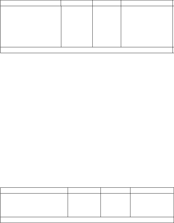
Table 1 Data for farmer’s problem.
Wheat Corn Sugar Beets
Yield (T/acre) 2.5 3 20
Planting cost ($/acre) 150 230 260
Selling price ($/T) 170 150 36 under 6000 T
10 above 6000 T
Purchase price ($/T) 238 210 –
Minimum require- 200 240 –
ment (T)
Total available land: 500 acres
73 w
4
= tons of sugar beets sold at the lower price.
The problem reads as follows:
min 150x
1
+ 230x
2
+ 260x
3
+ 238y
1
−170w
1
+ 210y
2
−150w
2
−36w
3
−10w
4
s. t. x
1
+ x
2
+ x
3
≤ 500 , 2.5 x
1
+ y
1
−w
1
≥ 200 ,
3 x
2
+ y
2
−w
2
≥ 240 , w
3
+ w
4
≤ 20x
3
,w
3
≤ 6000 ,
x
1
,x
2
,x
3
, y
1
,y
2
, w
1
,w
2
,w
3
,w
4
≥ 0 .
(1.1)
After solving (1.1) with his favorite linear program solver, the farmer obtains an
optimal solution, as in Table 2.
Table 2 Optimal solution based on expected yields.
Culture Wheat Corn Sugar Beets
Surface (acres) 120 80 300
Yield (T) 300 240 6000
Sales (T) 100 – 6000
Purchase (T) – – –
Overall profit: $118,600
This optimal solution is easy to understand. The farmer devotes enough land to
sugar beets to reach the quota of 6000 T. He then devotes enough land to wheat and
corn production to meet the feeding requirement. The rest of the land is devoted to
wheat production. Some wheat can be sold.
To an extent, the optimal solution follows a very simple heuristic rule: to allocate
land in order of decreasing profit per acre. In this example, the order is sugar beets
at a favorable price, wheat, corn, and sugar beets at the lower price. This simple
6 1 Introduction and Examples
heuristic would, however, no longer be valid if other constraints, such as labor re-
quirements or crop rotation, would be included.
After thinking about this solution, the farmer becomes worried. He has indeed
experienced quite different yields for the same crop over different years mainly be-
cause of changing weather conditions. Most crops need rain during the few weeks
after seeding or planting, then sunshine is welcome for the rest of the growing pe-
riod. Sunshine should, however, not turn into drought, which causes severe yield
reductions. Dry weather is again beneficial during harvest. From all these factors,
yields varying 20 to 25% above or below the mean yield are not unusual.
In the next sections, we study two possible representations of these variable
yields. One approach using discrete, correlated random variables is described in
Sections 1.1b. and 1.1c. Another, using continuous uncorrelated random variables,
is described in Section 1.1d.
The influence of price fluctuations, illustrated by the dramatic price increases in
2007, is discussed in Exercise 8.
b. A scenario representation
A first possibility is to assume some correlation among the yields of the different
crops. A very simplified representation of this would be to assume that years are
good, fair, or bad for all crops, resulting in above average, average, or below average
yields for all crops. To fix these ideas, “above” and “below” average indicate a yield
20% above or below the mean yield given in Table 1. For simplicity, we assume
that weather conditions and yields for the farmer do not have a significant impact on
prices.
The farmer wishes to know whether the optimal solution is sensitive to variations
in yields. He decides to run two more optimizations based on above average and
below average yields. Tables 3 and 4 give the optimal solutions he obtains in these
cases.
Again, the solutions in Tables 3 and 4 seem quite natural. When yields are high,
smaller surfaces are needed to raise the minimum requirements in wheat and corn
and the sugar beet quota. The remaining land is devoted to wheat, whose extra pro-
duction is sold. When yields are low, larger surfaces are needed to raise the mini-
mum requirements and the sugar beet quota. In fact, corn requirements cannot be
satisfied with the production, and some corn must be bought.
The optimal solution is very sensitive to changes in yields. The optimal surfaces
devoted to wheat range from 100 acres to 183.33 acres. Those devoted to corn
range from 25 acres to 80 acres and those devoted to sugar beets from 250 acres
to 375 acres. The overall profit ranges from $59,950 to $167,667.
Long-term weather forecasts would be very helpful here. Unfortunately, as even
meteorologists agree, weather conditions cannot be accurately predicted six months
ahead. The farmer must make up his mind without perfect information on yields.

1.1 A Farming Example and the News Vendor Problem 7
Table 3 Optimal solution based on above average yields (+ 20%).
Culture Wheat Corn Sugar Beets
Surface (acres) 183.33 66.67 250
Yield (T) 550 240 6000
Sales (T) 350 – 6000
Purchase (T) – – –
Overall profit: $167,667
Table 4 Optimal solution based on below average yields ( −20% ).
Culture Wheat Corn Sugar Beets
Surface (acres) 100 25 375
Yield (T) 200 60 6000
Sales (T) – – 6000
Purchase (T) – 180 –
Overall profit: $59,950
The main issue here is clearly on sugar beet production. Planting large surfaces
would make it certain to produce and sell the quota, but would also make it likely to
sell some sugar beets at the unfavorable price. Planting small surfaces would make
it likely to miss the opportunity to sell the full quota at the favorable price.
The farmer now realizes that he is unable to make a perfect decision that would be
best in all circumstances. He would, therefore, want to assess the benefits and losses
of each decision in each situation. Decisions on land assignment (x
1
,x
2
,x
3
) have
to be taken now, but sales and purchases (w
i
, i = 1,...,4, y
j
, j = 1,2) depend
on the yields. It is useful to index those decisions by a scenario index s = 1,2,3
corresponding to above average, average, or below average yields, respectively. This
creates a new set of variables of the form w
is
, i = 1,2,3,4, s = 1,2, 3andy
js
,
j = 1,2, s = 1,2, 3 . As an example, w
32
represents the amount of sugar beets sold
at the favorable price if yields are average.
Assuming the farmer wants to maximize long-run profit, it is reasonable for him
to seek a solution that maximizes his expected profit. (This assumption means that
the farmer is neutral about risk. For a discussion of risk aversion and alternative
utilities, see Chapter 2.) If the three scenarios have an equal probability of 1/3,the
farmer’s problem reads as follows:
8 1 Introduction and Examples
min 150x
1
+ 230x
2
+ 260x
3
−
1
3
(170w
11
−238y
11
+ 150w
21
−210y
21
+ 36w
31
+ 10w
41
)
−
1
3
(170w
12
−238y
12
+ 150w
22
−210y
22
+ 36w
32
+ 10w
42
)
−
1
3
(170w
13
−238y
13
+ 150w
23
−210y
23
+ 36w
33
+ 10w
43
)
s.t. x
1
+ x
2
+ x
3
≤ 500 , 3x
1
+ y
11
−w
11
≥ 200 ,
3.6x
2
+ y
21
−w
21
≥ 240 , w
31
+ w
41
≤ 24x
3
, w
31
≤ 6000 ,
2.5x
1
+ y
12
−w
12
≥ 200 , 3x
2
+ y
22
−w
22
≥ 240 ,
w
32
+ w
42
≤ 20x
3
, w
32
≤ 6000 , 2x
1
+ y
13
−w
13
≥ 200,
2.4x
2
+ y
23
−w
23
≥ 240, w
33
+ w
43
≤ 16x
3
,
w
33
≤ 6000, x, y,w ≥0 .
(1.2)
Such a model of a stochastic decision program is known as the extensive form of the
stochastic program because it explicitly describes the second-stage decision vari-
ables for all scenarios. The optimal solution of (1.2)isgiveninTable5.Thetop
line gives the planting areas, which must be determined before realizing the weather
and crop yields. This decision is called the first stage. The other lines describe the
yields, sales, and purchases in the three scenarios. They are called the second stage.
The bottom line shows the overall expected profit.
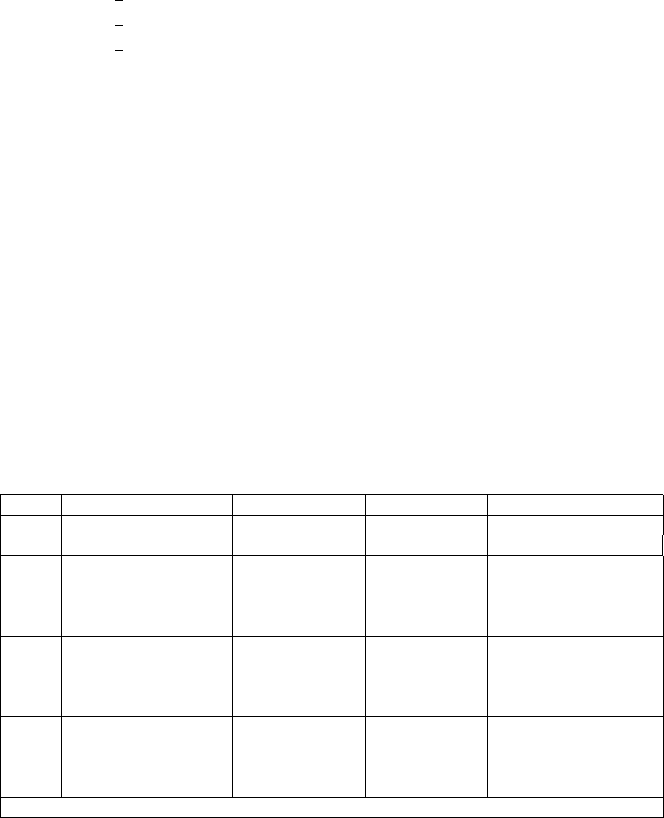
Table 5 Optimal solution based on the stochastic model (1.2).
Wheat Corn Sugar Beets
First Area (acres) 170 80 250
Stage
s = 1 Yield (T) 510 288 6000
Above Sales (T) 310 48 6000
(favor. price)
Purchase (T) – – –
s = 2 Yield (T) 425 240 5000
Average Sales (T) 225 – 5000
(favor. price)
Purchase (T) – – –
s = 3 Yield (T) 340 192 4000
Below Sales (T) 140 – 4000
(favor. price)
Purchase (T) – 48 –
Overall profit: $108,390
The optimal solution can be understood as follows. The most profitable decision
for sugar beet land allocation is the one that always avoids sales at the unfavorable
price even if this implies that some portion of the quota is unused when yields are
average or below average.
The area devoted to corn is such that it meets the feeding requirement when
yields are average. This implies sales are possible when yields are above average
1.1 A Farming Example and the News Vendor Problem 9
and purchases are needed when yields are below average. Finally, the rest of the land
is devoted to wheat. This area is large enough to cover the minimum requirement.
Sales then always occur.
This solution illustrates that it is impossible, under uncertainty, to find a solution
that is ideal under all circumstances. Selling some sugar beets at the unfavorable
price or having some unused quota is a decision that would never take place with a
perfect forecast. Such decisions can appear in a stochastic model because decisions
have to be balanced or hedged against the various scenarios.
The hedging effect has an important impact on the expected optimal profit. Sup-
pose yields vary over years but are cyclical. A year with above average yields is
always followed by a year with average yields and then a year with below average
yields. The farmer would then take optimal solutions as given in Table 3,thenTa-
ble 2,thenTable4, respectively. This would leave him with a profit of $167,667
the first year, $118,600 the second year, and $59,950 the third year. The mean profit
over the three years (and in the long run) would be the mean of the three figures,
namely $115,406 per year.
Now, assume again that yields vary over years, but on a random basis. If the
farmer gets the information on the yields before planting, he will again choose the
areas on the basis of the solution in Table 2, 3,or 4, depending on the information
received. In the long run, if each yield is realized one third of the years, the farmer
will get again an expected profit of $115,406 per year. This is the situation under
perfect information.
As we know, the farmer unfortunately does not get prior information on the
yields. So, the best he can do in the long run is to take the solution as given by
Table 5. This leaves the farmer with an expected profit of $108,390. The differ-
ence between this figure and the value, $115,406, in the case of perfect information,
namely $7016, represents what is called the expected value of perfect information
( EVPI ). This concept, along with others, will be studied in Chapter 4. At this intro-
ductory level, we may just say that it represents the loss of profit due to the presence
of uncertainty.
Another approach the farmer may have is to assume expected yields and always
to allocate the optimal planting surface according to these yields, as in Table 2.This
approach represents the expected value solution. It is common in optimization but
can have unfavorable consequences. Here, as shown in Exercise 1, using the ex-
pected value solution every year results in a long run annual profit of $107,240. The
loss by not considering the random variations is the difference between this and the
stochastic model profit from Table 5. This value, $108,390 −107,240=$1,150,is the
value of the stochastic solution ( VSS ), the possible gain from solving the stochastic
model. Note that it is not equal to the expected value of perfect information, and, as
we shall see in later models, may in fact be larger than the EVPI .
These two quantities give the motivation for stochastic programming in general
and remain a key focus throughout this book. EVPI measures the value of know-
ing the future with certainty while VSS assesses the value of knowing and using
distributions on future outcomes. Our emphasis will be on problems where no fur-
ther information about the future is available so the VSS becomes more practically
10 1 Introduction and Examples
relevant. In some situations, however, more information might be available through
more extensive forecasting, sampling, or exploration. In these cases, EVPI would
be useful for deciding whether to undertake additional efforts.
c. General model formulation
We may also use this example to illustrate the general formulation of a stochastic
problem. We have a set of decisions to be taken without full information on some
random events. These decisions are called first-stage decisions and are usually rep-
resented by a vector x . In the farmer example, they are the decisions on how many
acres to devote to each crop. Later, full information is received on the realization
of some random vector ξ . Then, second-stage or corrective actions y are taken.
We use boldface notation here and throughout the book to denote that these vectors
are random and to differentiate them from their realizations. We also sometimes
use a functional form, such as
ξ
(
ω
) or y(s) , to show explicit dependence on an
underlying element,
ω
or s .
In the farmer example, the random vector is the set of yields and the corrective
actions are purchases and sales of products. In mathematical programming terms,
this defines the so-called two-stage stochastic program with recourse of the form
min c
T
x + E
ξ
Q(x,ξ)
s. t. Ax = b ,
x ≥ 0 ,
(1.3)
where Q(x,ξ)=min{q
T
y | Wy = h −Tx,y ≥ 0}, ξ is the vector formed by the
components of q
T
, h
T
,and T ,and E
ξ
denote mathematical expectation with
respect to ξ . We assume here that W is fixed (fixed recourse). Reasons for this
restriction are explained in Section 3.1.
In the farmer example, the random vector is a discrete variable with only three
different values. Only the T matrix is random. A second-stage problem for one
particular scenario s can thus be written as
Q(x,s)=min {238y
1
−170w
1
+ 210y
2
−150w
2
−36w
3
−10w
4
}
s. t. t
1
(s)x
1
+ y
1
−w
1
≥ 200 ,
t
2
(s)x
2
+ y
2
−w
2
≥ 240 ,
w
3
+ w
4
≤t
3
(s)x
3
,
w
3
≤ 6000 ,
y,w ≥ 0 ,
(1.4)
where t
i
(s) represents the yield of crop i under scenario s (or state of nature s ).
To illustrate the link between the general formulation (1.3) and the example (1.4),
observe that in (1.4) we may say that the random vector ξ =(t
1
,t
2
,t
3
) is formed by

1.1 A Farming Example and the News Vendor Problem 11
the three yields and that ξ can take on three different values, say
ξ
1
,
ξ
2
,and
ξ
3
,
which represent (t
1
(1),t
2
(1),t
3
(1)) , (t
1
(2),t
2
(2),t
3
(2)) ,and (t
1
(3),t
2
(3),t
3
(3)) ,
respectively.
An alternative interpretation would be to say that the random vector
ξ
(s) in fact
depends on the scenario s , which takes on three different values
1
.
In this section, we have illustrated two possible representations of a stochastic
program. The form (1.2) given earlier for the farmer’s example is known as the ex-
tensive form. It is obtained by associating one decision vector in the second-stage
to each possible realization of the random vector. The second form (1.3)or(1.4)
is called the implicit representation of the stochastic program. A more condensed
implicit representation is obtained by defining Q(x)=E
ξ
Q(x,ξ) as the value func-
tion or recourse function so that (1.3) can be written as
min c
T
x + Q(x)
s. t. Ax = b ,
x ≥ 0 .
(1.5)
d. Continuous random variables
Contrary to the assumption made in Section 1.1b., we may also assume that yields
for the different crops are independent. In that case, we may as well consider a
continuous random vector for the yields. To illustrate this, let us assume that the
yield for each crop i can be appropriately described by a uniform random variable,
inside some range [l
i
,u
i
] (see Appendix A.2). For the sake of comparison, we may
take l
i
to be 80% of the mean yield and u
i
to be 120% of the mean yield so
that the expectations for the yields will be the same as in Section 1.1b. Again, the
decisions on land allocation are first-stage decisions because they are taken before
knowledge of the yields. Second-stage decisions are purchases and sales after the
growing period. The second-stage formulation can again be described as Q(x)=
E
ξ
Q(x,ξ) ,where Q(x,ξ) is the value of the second stage for a given realization of
the random vector.
Now, in this particular example, the computation of Q(x,ξ) can be separated
among the three crops due to independence of the random vector. (Note that this
separability property also holds in the discrete representation of Section 1.1b.)We
can then write:
E
ξ
Q(x,ξ)=
3
∑
i=1
E
ξ
Q
i
(x
i
,ξ)=
3
∑
i=1
Q
i
(x
i
) , (1.6)
where Q
i
(x
i
,ξ) is the optimal second-stage value of purchases and sales of crop i .
We are in fact in position to give an exact analytical expression for the second-
stage value functions Q
i
(x
i
) , i = 1,...,3 . We first consider sugar beet sales. For
1
Note that the decisions y
1
, y
2
, w
1
, w
2
, w
3
,and w
4
also depend on the scenario. This
dependence is not always made explicit. It appears explicitly in (1.7) but not in (1.4).

12 1 Introduction and Examples
agivenvalue t
3
(ξ) of the sugar beet yield, one obtains the following second-stage
problem:
Q
3
(x
3
,ξ)=min −36w
3
(ξ) −10w
4
(ξ)
s. t. w
3
(ξ)+w
4
(ξ) ≤t
3
(ξ)x
3
,
w
3
(ξ) ≤ 6000 ,
w
3
(ξ),w
4
(ξ) ≥ 0 .
(1.7)
The optimal decisions for this problem are clearly to sell as many sugar beets as
possible at the favorable price, and to sell the possible remaining production at the
unfavorable price, namely
w
3
(ξ)=min[6000,t
3
(ξ)x
3
] ,
w
4
(ξ)=max[t
3
(ξ)x
3
−6000,0] .
(1.8)
This results in a second-stage value of
Q
3
(x
3
,ξ)=−36min[6000,t
3
(ξ)x
3
] −10max[t
3
(ξ)x
3
−6000,0] .
We first assume that the surface x
3
devoted to sugar beets will not be so large
that the quota would be exceeded for any possible yield or so small that production
would always be less than the quota for any possible yield. In other words, we
assume that the following relation holds:
l
3
x
3
≤ 6000 ≤ u
3
x
3
, (1.9)
where, as already defined, l
3
and u
3
are the bounds on the possible values of t
3
(ξ) .
Under this assumption, the expected value of the second stage for sugar beet sales
is
Q
3
(x
3
)=E
ξ
Q
3
(x
3
,ξ
3
)
= −
6000/x
3
l
3
36tx
3
f (t)dt
−
u
3
6000/x
3
(216000 + 10tx
3
−60000) f (t)dt,
where f (t) denotes the density of the random yield t
3
(ξ) . Given the assumption
that this density is uniform over the interval [l
3
,u
3
] , one obtains, after some com-
putation, the following analytical expression
Q
3
(x
3
)=−18
(u
2
3
−l
2
3
)x
3
u
3
−l
3
+
13(u
3
x
3
−6000)
2
x
3
(u
3
−l
3
)
,
which can also be expressed as
Q
3
(x
3
)=−36
¯
t
3
x
3
+
13(u
3
x
3
−6000)
2
x
3
(u
3
−l
3
)
, (1.10)

1.1 A Farming Example and the News Vendor Problem 13
where
¯
t
3
denotes the expected yield for sugar beet production, which is
u
3
+l
3
2
for
a uniform density.
Note that assumption (1.9) is not really limiting. We can still compute the ana-
lytical expression of Q
3
(x
3
) for the other situations.
For example, if the surface x
3
is such that the production exceeds the quota
for any possible yield (l
3
x
3
> 6000) , then the optimal second-stage decisions are
simply
w
3
(ξ)=6000 ,
w
4
(ξ)=t
3
(ξ)x
3
−6000 , for all ξ .
The second-stage value for a given
ξ
is now
Q
3
(x
3
,
ξ
)=−216000 −10(t
3
(
ξ
)x
3
−6000)=−156000 −10t
3
(
ξ
)x
3
,
and the expected value is simply
Q
3
(x
3
)=−156000−10
¯
t
3
x
3
. (1.11)
Similarly, if the surface devoted to sugar beets is so small that for any yield the
production is lower than the quota, the second-stage value function is
Q
3
(x
3
)=−36
¯
t
3
x
3
. (1.12)
We may therefore draw the graph of the function Q
3
(x
3
) for all possible values of
x
3
as in Figure 1. Note that with our assumption of
¯
t
3
= 20 , we would then have
the limits on x
3
in (1.9) as 250 ≤ x
3
≤ 375 .
Fig. 1 The expected recourse value for sugar beets as a function of acres planted.
We immediately see that the function has three different pieces. Two of these pieces
are linear and one is nonlinear, but the function Q
3
(x
3
) is continuous and convex.
This property will be proved when we consider the generalization of this problem,