Daniels M.J., Hogan J.W. Missing Data in Longitudinal Studies: Strategies for Bayesian Modeling and Sensitivity Analysis
Подождите немного. Документ загружается.

10 MOTIVATING EXAMPLES
−2000 −1000 0 1000
0 500 1000 1500 2000
time since HAART initiation
CD4
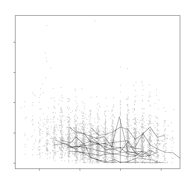
Figure 1.4 HER Study: Plot of CD4 vs. time for 393 HIV infected women who
received HAART during their enrollment in HERS. Horizontal axis is centered at
time of the first visit where receipt of HAART is reported.
1.5.4 Data analyses
An analysis of these data is given in Chapter 6. The nonlinearity of the time
trend motivates a flexible approach to modeling; we use penalized splines
under MAR to characterize the population CD4 curve, with emphasis on
the importance of choosinganappropriate variance-covariance model and its
effect on the fitted curve.

OASIS STUDY 11
1.6 Clinical trial of smoking cessation among substance abusers:
OASIS study
1.6.1 Study and data
The OASIS Trial is an NIH-funded study designed to compare standard (ST)
vs. enhanced (ET) counseling interventions for smoking cessation among al-
coholics. The trial enrolled 298 individuals, randomized to standard vs. more
intensive counseling. Assessment of smoking status was made at 1, 3, 6, and
12 months following randomization. Previous analyses of these data appear
in Lee et al. (2007).
1.6.2 Questions of interest
Theprimary goal of our analysis is comparison of smoking cessation rates at
12 months by treatment randomization (i.e., intention to treat effect).
Table 1.3 OASIS Trial: number (proportion) quit, smoking and missing at each
month. S/(Q + S) denotes empirical smoking rate among those still in follow-up;
(S + M)/(Q + S + M ) denotes empirical smoking rate after counting missing values
as smokers. ET = enhanced intervention, ST = standard intervention.
Month
Treatment 1 3 6 12
ET Quit 26 (.18) 13 (.09) 17 (.11) 16 (.11)
(n = 149) Smoking 123 (.83) 70 (.47) 63 (.42) 51 (.34)
Missing — 66 (.44) 69 (.46) 82 (.55)
S
Q + S
.83 .84 .79 .76
S + M
Q + S + M
.83 .91 .89 .89
ST Quit 23 (.15) 14 (.09) 15 (.10) 11 (.07)
(n = 149) Smoking 126 (.85) 80 (.54) 78 (.52) 78 (.52)
Missing — 55 (.37) 56 (.38) 60 (.40)
S
Q + S
.85 .85 .84 .88
S + M
Q + S + M
.85 .91 .90 .93

12 MOTIVATING EXAMPLES
1.6.3 Missing data
Dropout rate was relatively high in the OASIS study (40% on ST, 55% on ET).
Table 1.3 summarizes proportion quit, smoking, and missing at each month,
stratified by treatment arm, and includes two commonly used estimates of
overall smoking rate.Thefirst is derived using only those still in follow-up, and
the second assumes those with missing observations are smokers.
∗
In Table 1.4
the association between status at times t
j−1
and t
j
(for j =2, 3, 4) indicates
that smoking status at t
j−1
is predictive of dropout at t
j
,andmotivates the
use of models that assume MAR at a minimum.
Table 1.4 OASIS Trial: numberandproportion of transitions from status at mea-
surement times t
j−1
to t
j
(with t
j
corresponding to months 1, 3,6,and12for
j =1, 2, 3, 4), stratified by treatment. Figures in parentheses are row proportions.
ET = enhanced intervention, ST = standard intervention.
Status Status at t
j
(j =2, 3, 4)
Treatment at t
j−1
Quit Smoking Missing Total
Quit 26 (.46) 21 (.38) 9 (.16) 56
ET Smoking 18 (.07) 152 (.59) 86 (.34) 256
Missing 2 (.01) 11 (.08) 122 (.90) 135
Quit 24 (.46) 17 (.33) 11 (.21) 52
ST Smoking 12(.04) 204 (.72) 68 (.24) 284
Missing 4 (.04) 15 (.14) 92 (.83) 111
1.6.4 Data analyses
These data are analyzed in detail in Section 10.3, using both MAR and MNAR
models. The first analysis uses a pattern mixture model where, conditional on
dropout time, the longitudinal smoking outcomes follow a Markov transition
model. The model is fit under MAR assumptions, then elaborated to allow
for MNAR mechanisms. Sensitivity analyses and the use of informative priors
elicited from experts are illustrated.
We also use a selection model approach, allowing for MNAR dropout. The
two models are compared in terms of inference about treatment effect and
assumptions about missing data.
∗
In our analyses of these data, we make a simplifying assumption that those with missing
outcome at month 1 are smokers.

PEDIATRIC AIDS TRIAL 13
1.7 Equivalence trial of competing doses of AZT in HIV-infected
children: Protocol 128 of the AIDS Clinical Trials Group
1.7.1 Study and data
ACTG 128 is a randomized equivalence trial of high vs. low dose of AZT for
thetreatment of HIV in children (Brady et al., 1998). The trial enrolled 426
children and randomized them to a regimen of either 180mg or 90mg AZT six
times daily. Because AZT is associated with potentially harmful side effects
and drug toxicity, the trial was designed to provide information on whether the
lower dose provided efficacy comparable to the high dose while reducing the
rate of side effects. The key clinical outcomes are CD4 cell count, scheduled
for measurement every 3 months, and neurocognitive test results, scheduled
for measurement every 6 months. Our focus here is on CD4 cell counts; both
the CD4 and neurocognitive outcomes have been been analyzed elsewhere,
with attention to handling dropout and noncompliance; see Hogan and Laird
(1996); Hogan and Daniels (2002), and Hogan et al. (2004a).
050100 150 200
02468
High dose
Weeks from baseline
log CD4
050100 150 200
02468
Low Dose
Weeks from baseline
log CD4
Figure 1.5 Pediatric AIDS Trial: CD4 count vs. time for all individuals, stratified
by treatment, with a subsample of individual trajectories highlighted.
14 MOTIVATING EXAMPLES
1.7.2 Questions of interest
The primary objective of our analyses is comparison of change in CD4 count
from baseline to the end of the study, using the intention to treat principle;
that is, we seek to compare change in CD4 among all participants randomized
to high or low dose AZT.
1.7.3 Missing data
Dropout occurs for various reasons, including lack of treatment effect and drug
toxicity. A key feature of this study is that dropout time is measured on a
continuum, which requires some added flexibility in the modeling process. For
purposes of keeping the example straightforward, wedonotuseinformation
about reason for dropout in our analyses, but see Hogan and Laird (1996) and
Hogan and Daniels (2002) for analyses that do. Figure 1.5 shows CD4 counts
aggregated over all individuals, with a subsample of individual trajectories
highlighted. The plot suggests that dropouts (those with shorter trajectories)
tend to have a lower CD4 count at baseline and a more pronounced negative
slope over time.
1.7.4 Data analyses
These data are analyzed in Section 10.4 using amixtureofvarying coefficient
models (Hogan et al., 2004a). The modeling approach allows regression coef-
ficients such as slope over time to vary as smooth functions of dropout times.
The conditional distribution of CD4 given dropout is then averaged over the
dropout distribution, which can be modeled nonparametrically. The results of
our analysis are compared to thestandard random effects approach.

CHAPTER 2
Regression Models
for Longitudinal Data
2.1 Overview
This chapter reviews some modern approaches to formulation and interpre-
tation of regression models for longitudinal data. Section 2.2 outlines nota-
tion for longitudinal data and describesbasicregression approaches. In Sec-
tion 2.3 we describe the generalized linear model (GLM) for univariate data,
which forms the basis of many regression models for longitudinal data. Sec-
tions 2.4 and 2.5 describe different approaches to regression modeling based
on whether the mean is specified directly, in terms of marginal means; or con-
ditionally, in terms of latent variables, random effects, or response history.
Many conditionally specified models are multilevel models that partition the
variance-covariance structureinanaturalway,leading to low dimensional
parameterizations.
In Section 2.6 we focus on semiparametric models highlighting those that
permit flexibility in modeling time trends and allow covariate effects to vary
smoothly with time (e.g., varying coefficient models). Finally, Section 2.7 re-
views key issues in the interpretation oflongitudinal regression models, high-
lighting longitudinal vs. cross-sectional effects and key assumptions about
time-varying covariates.
The literature on regression models forlongitudinal data is vast, and we
make no attempt to be comprehensive here. Our review is designed to highlight
predominant approaches to regression modeling, emphasizing those models
used in later chapters. Forrecent accounts, readers are referred to Davidian
and Giltinan (1998); Verbeke and Molenberghs (2000); Diggle et al. (2002);
Fitzmauriceetal. (2004); Laird (2004); Weiss (2005); Hedeker and Gibbons
(2006) and Molenberghs and Verbeke (2006).
2.2 Preliminaries
2.2.1 Longitudinal data
Appealing to first principles, one can think of longitudinal data as arising
from the joint evolution of response and covariates,
{Y
i
(t), x
i
(t):t ≥ 0}.
15
16 REGRESSION MODELS
If the process is observed at a discrete set of time points T = {t
1
,...,t
J
}
that is common to all individuals, the resulting response data can be written
as a J × 1vector
Y
i
= {Y
i
(t):t ∈ T }
=(Y
i1
,...,Y
iJ
)
T
.
The covariate process {x
i
(t):t ≥ 0} is 1 × p.Attimet
j
,theobserved
covariates are collected in the 1 × p vector
x
ij
= x
i
(t
j
)
=(x
i1
(t
j
),...,x
ip
(t
j
))
=(x
ij1
,...,x
ijp
).
Hence the full collection of observed covariates is contained in the J ×p matrix
X
i
=
x
i1
x
i2
.
.
.
x
iJ
.
When the set of observation times is common to all individuals, we say the
responses are balanced or temporally aligned.Itissometimes the case that
observation times are unbalanced,ortemporally misaligned,inthatthey vary
by subject. In this case the set T is indexed by i,suchthat
T
i
= {t
i1
,...,t
iJ
i
},
and the dimensions of Y
i
and X
i
are J
i
× 1andJ
i
× p,respectively.
In regression, we are interested in characterizing the effect of covariates X
on a longitudinal dependent variable Y .Formally,wewishtodrawinference
about the joint distribution of the vector Y
i
conditionally on X
i
.Likelihood-
based regression models for longitudinal data require a specification of this
joint distribution using a model p(y | x, θ). The parameter θ typically is a
finite-dimensional vector of parameters indexing the model; it might include
regression coefficients, variance components, and parameters indexing serial
correlation.
The joint distribution of responses canspecifieddirectly or conditionally.
In this chapter we differentiate models on how the mean is specified. A model
with a directly specified mean characterizes E(Y | x)without resorting to
latent structures such as random effects. Models with conditionally specified
means include Markov models and various types of multilevel models, where
the mean is given conditionally on previous responses or on random effects
that reflect aspects of the joint response distribution. Mostly, we deal with
conditionally specified models that use a multilevel format, for example involv-
ing subject-specific random effects or latent variables b to partition within-
PRELIMINARIES 17
and between-subject variation. The usual strategy is to specify a model for
the joint distribution of responses and random effects, factored as
p(y, b | x)=p(y | b, x) p(b | x).
The distribution of interest, p(y | x), is obtained by integrating over b.For
example, if the conditional mean is given by a function like
E(Y | x, b)=g(xβ + b),
then
E(Y | x)=
g(xβ + b) p(b | x) db,
which may not always take a closed form.
2.2.2 Regression models
As we review several different regression models, the intent is to give the
reader a sense of the rich variety of models that can be used to characterize
longitudinal data, and to demonstrate how these fit coherently into a single
framework. As a result, missing data strategies described in later chapters
can be applied very generally. Methods described here will be familiar to
those with experience analyzing longitudinal data (e.g., multivariate normal
regression model, random effects models), but others represent fairly new
developments. Examples include marginalized transition models (Heagerty,
2002), varying coefficient models (Zhang, 2004), and regression splines (Eilers
and Marx, 1996; Lin and Zhang, 1999; Ruppert et al., 2003). Here we focus on
specification and interpretation;Chapter 3 covers various aspects of inference.
Because many regression models for longitudinal data have their founda-
tion in the generalized linear model (GLM) for cross-sectional data (McCul-
lagh and Nelder, 1989), our review begins with a concise description of GLMs.
Coverage of models for longitudinal data begins with random effects models;
these build directly on the GLM structure by introducing individual-level ran-
dom effects to capture between-subject variation. Conditional on the random
effects, within-level variation can be described by a simpler model, such as a
GLM. Random effects models are very attractive in that they naturally parti-
tion variation in the dependent variable into its between- and within-subject
components, and they can be used to model both balanced and unbalanced
data. At the same time, there is sometimes the disadvantage that the implied
marginal distributions of responses can be opaque.
Directly specified models have a natural construction when the error dis-
tribution is multivariate normal; for binary, count, and other discrete data,
the choice of an appropriate joint distribution is less obvious. Our review
touches on some recent developments for discrete longitudinalresponses, such
as the marginalized transition model (Heagerty, 2002). For a detailed review
18 REGRESSION MODELS
of likelihood-based models of multivariate discrete response, see Chapter 11 of
Diggle et al. (2002), Chapter 7 of Laird (2004), and Chapter 11 of Fitzmaurice
et al. (2004).
For all mo dels covered in the first part of this chapter, E(Y | x)takesa
known functional form, usually linear in some transformed scale. Section 2.6
describes models in which the regression function is unknown but can be at
least partially specified in terms of unspecified smooth functions. The latter
type of model is typically called semiparametric,because one or more com-
ponents of the regression function are left unspecified, while distributional
assumptions are made about the error structure. Nonlinear and semipara-
metric models have a close connection to the GLM structure; we emphasize
that connection and illustrate that regression models as a whole can be very
generally characterized (Hastie and Tibshirani, 1990; Ruppert et al., 2003).
The final element of our review concerns interpretation of covariate ef-
fects in longitudinal models. Because the response and covariates change with
time, models of longitudinal data afford the opportunity to infer both within-
andbetween-subject covariate effects; however the importance of underlying
assumptions to the interpretation of covariate effects should not be underesti-
mated. Section 2.7 discusses three key aspects of interpretation and specifica-
tion for longitudinal models: cross-sectional vs. longitudinal effects of a time-
varying covariate, marginal (population-averaged) vs. conditional (subject-
specific) covariate effects, and assumptions governing the use of time-varying
covariates.
2.2.3 Full vs. observed data
The distinction between full and observed data is particularly important when
drawing inference from incomplete longitudinal data. Throughout Chapters 2
and 3, the models refer to a full-data distribution.
We define the full data as those observations intended to be collected on a
pre-specified interval, such as [0,T]. For example, if intended collection times
t
1
,...,t
J
are common to all individuals, then the full response and covariate
data are (Y
i1
, X
i1
),...,(Y
iJ
, X
iJ
), where Y
ij
= Y
i
(t
j
)andX
ij
= X
i
(t
j
). In
Chapter 5 we expand the definition of full data to include random variables
such as dropout time that characterize the missing data process.
In most applications, interest lies intheeffect of covariates on the mean
structure. When data are fully observed,thevarianceand covariance models
can frequently be treated as nuisance parameters. Correct specification of
variance and covariance allows more efficient use of the data, but it is not
always necessary for obtaining proper inferences about mean parameters.
When data are not fully observed, variance-covariance specification takes
on heightened importance because missing data will effectively be imputed or
extrapolated from observed data, based on modeling assumptions. For longi-
GENERALIZED LINEAR MODELS 19
tudinal data, unobserved responses will be imputed from observed responses
for the same individual; the assumed correlation structure will usually dictate
(at least in part) the functional form of the imputation. This theme recurs
throughout the book, and therefore our review pays particular attention to
aspects of variance-covariance specification.
2.2.4 Additional notation
Random variables and their realizations are denoted by Roman letters (e.g.,
X, x), and parameters are representedbyGreek letters (e.g., α, θ). Vector-
and matrix-valued random variables and parameters are represented using
boldface (e.g., x, Y , β, Σ). For any matrix or vector A,weuseA
T
to denote
transpose. If A is invertible, then A
−1
is its inverse, |A| is its determinant,
and L = A
1/2
is the lower triangular matrix square root (Cholesky factor)
such that LL
T
= A.Aq-dimensional identity matrix is denoted I
q
and a
diagonal matrix by diag(a), where a is thevector of diagonal elements. The
parameterizations of specific probability distributions used in the text can be
found in the Appendix.
2.3 Generalized linear models for cross-sectional data
The generalized linear model (GLM) forms the foundation for many ap-
proaches to regression with multivariate responses, such as longitudinal or
clustered data. Models such as random effects or mixed effects models, latent
variable and latent class models, and regression splines, all highly flexible and
general, are based on the GLM framework. Moment-based methods such as
generalized estimating equations (GEE) also follow directly from the GLM
forcross-sectional data (Liang and Zeger, 1986).
The GLM is a regression modelforadependent variable Y arising from
the exponential family of distributions
p(y | θ, ψ)=exp{(yθ − b(θ)) /a(ψ)+c(y, ψ)} ,
where a, b,andc are known functions, θ is the canonical parameter,andψ
is a scale parameter.Theexponential family includes several commonly used
distributions, such as normal, Poisson, binomial, and gamma. It can be readily
shown that
E(Y )=b
(θ)
var(Y )=a(ψ)b
(θ),
where b
(θ)andb
(θ)arefirstandsecond derivatives of b(θ)withrespect to
θ (see McCullagh and Nelder, 1989, Section 2.2.2 for details).
The effect of covariates x
i
=(x
i1
,...,x
ip
)canbemodeledbyintroducing