Allman E.S., Rhodes J.A. Mathematical Models in Biology: An Introduction
Подождите немного. Документ загружается.

156 Modeling Molecular Evolution
0 50 100 150 200 250 300 350 400
0
0.1
0.2
0.3
0.4
0.5
0.6
0.7
0.8
t
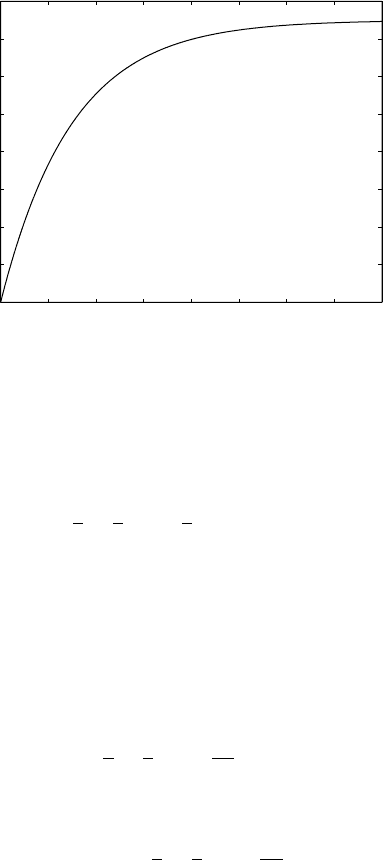
p(t) = 3/4 - (3/4)(1-4α/3)
t
Figure 4.1. The Jukes-Cantor model, α = .01: Fraction of differing sites at time t .
and computed the entries of M
t
for t = 0, 1, 2, 3,.... The diagonal entries
of M
t
turned out to all be
1
4
+
3
4
1 −
4
3
α
t
.
Now, the diagonal entries of M
t
give conditional probabilities that the base
at time t is the same as the base at time 0. In other words, they indicate the
probability of observing no change when the site at time 0 is compared with
the site at time t. Because all these diagonal entries are equal, this means that
at time step t we would expect to observe that the fraction of sites that agreed
with their initial base was given by the formula
q(t) =
1
4
+
3
4
1 −
4α
3
t
.
The fraction of sites that are different, then, will be
p(t) = 1 − q(t) =
3
4
−
3
4
1 −
4α
3
t
.
Why could you also get the formula for p(t) by adding the three off-
diagonal entries in any column of M
t
?
In the graph of p(t) in Figure 4.1, we of course see that p(0) = 0, because
at time t = 0, no substitutions have yet occurred. More interestingly, we see

4.5. Phylogenetic Distances 157
that the fraction of sites that differ from their original base gradually increases
with t, approaching the value
3
4
. This fraction never exceeds
3
4
, however.
Even if so much mutation has occurred that the two sequences appear
to be completely unrelated, you would expect to find agreement at
1
4
of
the sites. Why?
The graph also illustrates that, for each time t , p(t ) has a different value.
This means that given any value 0 ≤ p ≤ 3/4, we should be able to find
a t with p(t) = p. That is, from the proportion of sites that differ between
two sequences, we should be able to recover the number of elapsed time steps
(assuming we know α). For real sequence data, p is easily estimated, although
the elapsed time t and the mutation rate α usually are not known. Recovering
them from data is now our goal.
The Jukes-Cantor distance. Suppose we have records of an original
DNA sequence and a mutated version of it from some later time. Suppose
we also believe the Jukes-Cantor model describes the mutation process that
occurred, but we do not know either the mutation rate α or the number of
elapsed time steps t.
From the DNA sequence data, we can estimate p = p(t) by comparing
many sites before and after mutation and using the proportion of sites that
disagree in the two sequences as an estimate. For instance, if the original
sequence were AT T GAC and the final one AT GGCC, we would estimate
p(t) = 2/6 ≈ .333. Of course with real data, it is best to have much longer
DNA sequences so that we have more confidence in our estimate.
With p = p(t) estimated, how do we recover information on the mutation
rate α and the amount of elapsed time t? Since
p =
3
4
−
3
4
1 −
4
3
α
t
,
solving for t yields
t =
ln
1 −
4
3
p
ln
1 −
4
3
α
. (4.7)
To go further, we need to realize that our choice of a step size for time in
formulating our model affects both the value of the mutation rate α, and the
number of elapsed time steps between ancestor and descendent. We cannot
really expect to recover both of these. However, the product of the two does
158 Modeling Molecular Evolution
have a meaning that is more intrinsic to what we are modeling: Let
d = tα
= (no. of time steps)(mutation rate)
= (no. of time steps)(no. of substitutions per site/time step)
= (expected no. of substitutions per site during the elapsed time).
We emphasize that this expected number of substitutions includes even those
we do not observe because they are hidden by subsequent substitutions.
To extract d = tα from Eq. (4.7), we must use an approximation. Now
ln(1 + x) ≈ x when x is near 0 (see the Problems section). Furthermore, we
can be sure −
4
3
α is near 0 if we assume that we have chosen a time step that
is very small, so that the mutation rate per time step, α, is also very small.
Thus,
ln
1 −
4
3
α
≈−
4
3
α.
Substituting this into Equation (4.7) gives
t ≈
ln
1 −
4
3
p
−
4
3
α
≈−
3
4α
ln
1 −
4
3
p
,
or
d = tα ≈−
3
4
ln
1 −
4
3
p
.
If our time steps are made smaller, so the mutation rate α is also smaller, the
approximation used for the logarithm is increasingly accurate. We therefore
define the Jukes-Cantor distance between DNA sequences S
0
and S
1
as
d
JC
(S
0
, S
1
) =−
3
4
ln
1 −
4
3
p
,
where p is the fraction of sites that disagree in comparing S
0
with S
1
. Provided
the Jukes-Cantor model accurately describes the evolution of one sequence
into another, it is an estimate of the total number of substitutions per site that
occurred during the evolution.
“Distance” here is an abstract notion of how different the sequences are
because of mutations. Recall that if the mutation rate is constant over an evo-
lutionary history, we say there is a molecular clock. Provided a molecular

4.5. Phylogenetic Distances 159
clock hypothesis is valid, the distance computed here is proportional to the
amount of elapsed time, with the constant of proportionality being the muta-
tion rate. Thus, the distance can be thought of as a measure of how much time
was required for one sequence to mutate into the other. If the molecular clock
hypothesis does not hold, it is still a reconstruction of the average number
of substitutions that occurred at any one site. The larger it is, the greater the
evolutionary change.
Although we were unable to recover either the mutation rate α or the num-
ber of elapsed time periods t by themselves, we could at least recover the
product of the two from comparing sequences. If there is some other data
(such as a geological record) suggesting the time involved, then the mutation
rate can be found from d
JC
. This is one way that real DNA mutation rates are
estimated.
Example. Consider the two 40-base sequences at the end of Section 4.3.
From Table 4.1, we find that 11 of the sites have undergone a substitution, so
p = 11/40 = .2750. Thus,
d
JC
(S
0
, S
1
) =−
3
4
ln
1 −
4
3
11
40
≈ .3426.
Therefore, while we observed .2750 substitutions per site on average, we
estimate that in the course of evolution .3426 substitutions per site occurred.
Hidden mutations account for the difference.
The Kimura distances. Given any Markov model of base substitution, we
could hope to imitate the steps above to derive an appropriate formula recon-
structing the amount of mutation that has occurred. For the Kimura models,
you will find an exercise that steps you through the procedure. The final for-
mula for the Kimura 3-parameter model is
d
K 3
=−
1
4
(
ln(1 − 2β − 2γ ) + ln(1 − 2β − 2δ) + ln(1 − 2γ − 2δ)
)
,
where β, γ , and δ are estimates of parameters for a Kimura 3-parameter
matrix describing the mutation of the initial sequence to the final.
Of course, if γ = δ, this also gives a distance for the Kimura 2-parameter
model. In that case, β is the probability of a transition, while γ + δ = 2γ
is the probability of a transversion. Thus, if from sequence data we estimate
the probability of a transition p
1
by counting all transitions and dividing by
the length of the sequence, and the probability of a transversion p
2
similarly,
160 Modeling Molecular Evolution
we have
d
K 2
=−
1
2
ln(1 − 2 p
1
− p
2
) −
1
4
ln(1 − 2 p
2
).
If sequence data seems to indicate that transitions and each transversion
type did not proceed at equal rates, then the Jukes-Cantor model is a poor
one, and so the Kimura distance formulas are better choices for estimating
the total amount of mutation.
Additive and symmetric distances: Log-det. The distance formulas
given so far assume the data are consistent with either the Jukes-Cantor model
or a Kimura 2- or 3-parameter model. Because these models do not necessar-
ily describe all sequence data well, it is natural to ask for a distance formula
for the general Markov model.
To motivate such a formula, we will not focus on reconstructing the total
number of base substitutions that occurred, but rather on a property shared
by both the Jukes-Cantor and Kimura distances.
This property concerns the behavior of the distance formula when we con-
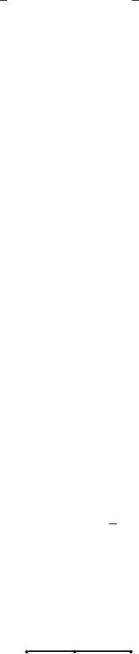
sider two successive mutation processes. Imagine an ancestral sequence S
0
from which has evolved S
1
, from which in turn has evolved S
2
, as shown
schematically in Figure 4.2.
Let M
0→1
= M(α
1
) and M
1→2
= M(α
2
) be two Jukes-Cantor matrices de-
scribing the two mutation processes as shown. Then, we can calculate a mu-
tation matrix M
0→2
for the full passage from S
0
to S
2
as the product
M
0→2
= M
1→2
M
0→1
.
Why are the matrices multiplied in this order?
A short calculation shows that M
0→2
is also a Jukes-Cantor matrix,
M
0→2
= M(α
3
), with
α
3
= α
1
+ α
2
−
4
3
α
1
α
2
.
As part of the Jukes-Cantor model, suppose the base distribution for each
of S
0
, S
1
, and S
2
is the equilibrium (1/4, 1/4, 1/4, 1/4). Then, in passing
from one sequence to the next by the Jukes-Cantor matrices M(α
i
), we find
S
0
S
1
S
2
M
01
M
12
→
→
Figure 4.2. Three sequences in evolutionary order.

4.5. Phylogenetic Distances 161
the fraction of sites that change is p = α
i
, and so the Jukes-Cantor distances
are
M(α
1
): −
3
4
ln
1 −
4
3
α
1
M(α
2
): −
3
4
ln
1 −
4
3
α
2
M(α
1
)M(α
2
) = M(α
3
): −
3
4
ln
1 −
4
3
(α
1
+ α
2
−
4
3
α
1
α
2
)
.
But a little algebra shows
−
3
4
ln
1 −
4(α
1
+ α
2
−
4
3
α
1
α
2
)
3
=
−
3
4
ln
1 −
4α
1
3
+
−
3
4
ln
1 −
4α
2
3
.
This means that multiplying two Jukes-Cantor matrices corresponds to adding
the associated distances.
We can see why this had to be the case if we recall that the Jukes-Cantor
distance is recovering the total number of substitutions per site that must have
occurred, including hidden ones. If we imagine a sequence mutating first
according to one matrix and then the other (i.e., according to the product of
the matrices), then the total number of substitutions per site would be the sum
of those described by each individual matrix.
Returning to the general Markov model, we would like a definition of
distance between sequences that has the additive property that
d(S
0
, S
2
) = d(S
0
, S
1
) + d(S
1
, S
2
)
in situations described by Figure 4.2.
To define such a distance, suppose F is the 4 × 4 frequency array obtained
by comparing sites in sequences S
0
and S
1
. Let f
0
and f
1
be the frequency
vectors for the bases in S
0
and S
1
, respectively. For instance, F might be
the entries in Table 4.1 with f
0
and f
1
its column and row sums. Then, one
version of the log-det distance (also called the paralinear distance in this
form) between S
0
and S
1
is defined by
d
LD
(S
0
, S
1
) =−
1
4
ln
(
det(F)
)
−
1
2
ln(g
0
g
1
)
,
where g
i
is the product of the 4 entries in f
i
. Recall from Chapter 2 that
“det” denotes the determinant of a matrix. Because the argument for why this
162 Modeling Molecular Evolution
distance is additive depends on some knowledge of linear algebra beyond this
text, we leave it to the exercises.
The meaning of the log-det distance is harder to interpret than the other
distances we have discussed. Unlike those, it usually is not just the total
number of mutations per site that must have occurred over the evolutionary
history. Still, you should think of it as some measure of the amount of mutation
that has occurred. In special circumstances, such as when the Jukes-Cantor
or Kimura models apply exactly, it gives the same result as they do, as you
will also see in the exercises.
The key fact that all the phylogenetic distances we have discussed are addi-
tive will be extremely useful in the next chapter, when we turn to constructing
phylogenetic trees relating many species.
Another useful property of all of these distances is symmetry. Although
we thought of having ancestral and descendent sequences in discussing the
various distances, in fact none of the final formulas depend on knowing which
one of the sequences was the ancestral one. For instance, the Jukes-Cantor
distance is calculated from first finding the fraction of sites that differ in the
two sequences. If we had the same sequences, but switched which one we
imagined was ancestral, we would calculate exactly the same distance. This
means
d(S
0
, S
1
) = d(S
1
, S
0
).
This property will also be very valuable to us, because usually we do not have
an ancestral sequence and a descendent one, but rather two descendents. In
the exercises, you will see how symmetry helps us use a distance formula in
this circumstance.
Problems
4.5.1. Calculate d
JC
(S
0
, S
1
) for the two 40-base sequences
S
0
: CT AGGCT T ACG ATT ACG AGGATCC AAATGGC ACC AATGCT
S
1
: C T ACGCT T ACG AC AACG AGG AT CCG AAT GGC ACC AT T GCT.
4.5.2. Ancestral and descendent sequences of 400 bases were simulated
according to the Jukes-Cantor model. A comparison of aligned sites
gave the frequency data in Table 4.7.
a. Compute the Jukes-Cantor distance to 10 decimal digits, showing
all steps.

4.5. Phylogenetic Distances 163
Table 4.7. Frequencies of S
1
= i
and S
0
= j in 400-Site Sequence
Comparison
S
1
\S
0
AGCT
A 90332
G 37982
C 2 4 96 5
T 51394
b. Compute the Kimura 2-parameter distance to 10 decimal digits,
showing all steps.
c. Are the answers to parts (a) and (b) identical? Explain.
4.5.3. Ancestral and descendent sequences of 400 bases were simulated
according to the Kimura 2-parameter model with γ = β/5. A com-
parison of aligned sites gave the frequency data in Table 4.8.
a. Compute the Jukes-Cantor distance to 10 decimal digits, showing
all steps.
b. Compute the Kimura 2-parameter distance to 10 decimal digits,
showing all steps.
c. Which of these is likely to be a better estimate of the number of
substitutions per site that actually occurred? Explain.
4.5.4. Compute the Kimura 3-parameter and log-det (paralinear) distance
for the sequences of the last two problems.
4.5.5. Graph d
JC
as a function of p.
a. Why does d
JC
= 0 if two sequences are identical?
b. Why does d
JC
not make sense if two sequences differ in 3/4or
more of the sites? Should this cause problems when trying to use
the formula on real data?
Table 4.8. Frequencies of S
1
= i
and S
0
= j in 400-Site Sequence
Comparison
S
1
\S
0
AGCT
A 92 15 2 2
G 13 84 4 4
C 0 1 77 16
T 4 2 14 70
164 Modeling Molecular Evolution
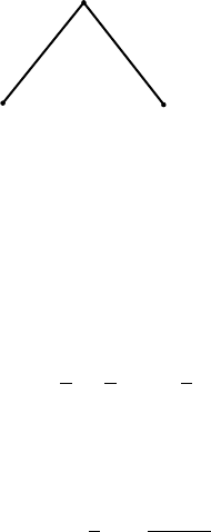
S
0
S
1
S
2
Figure 4.3. An evolutionary tree.
c. Explain in biological terms why, if two sequences differ in just
under 3/4 of the sites, the value of d
JC
should be very large.
4.5.6. Complete the gaps in the derivation of the formulas for d
JC
in the text
by doing all the necessary algebra on the equation
p =
3
4
−
3
4
1 −
4
3
α
t
to find the formula in Eq. (4.7) for t in terms of p and α.
4.5.7. The Jukes-Cantor distance formula is sometimes stated as
d
JC
=−
3
4
ln
4q − 1
3
,
where q is the proportion of bases that are the same in the “before”
and “after” sequences. Derive this formula from the one in the text.
4.5.8. Give numerical evidence that the approximation ln(1 + x) ≈ x is
valid for small x by making a table of values of x and ln(1 + x)
for x close to 0. Give graphical evidence by plotting y = ln(1 + x)
and y = x.
4.5.9. (Calculus) Show the approximation ln(1 + x) ≈ x is valid for x near
0 by using calculus to find the tangent line approximation to y =
ln(1 + x) at the point where x
0
= 0.
4.5.10. In practice, when applying a distance formula to real DNA sequence
data, it is uncommon to have sequences for both an ancestor and a
descendent. Instead, we usually have two descendent DNA sequences
S
1
and S
2
that mutated from a common, yet unknown, ancestral se-
quence S
0
, as in Figure 4.3. From the data, we can only compute
d(S
1
, S
2
). Show that, for an additive, symmetric distance, this is the
same as d(S
0
, S
1
) + d(S
0
, S
2
).
4.5.11. When transitions are more frequent than transversions, the Kimura
2-parameter distance often gives a larger value than the Jukes-Cantor

4.5. Phylogenetic Distances 165
distance. Explain this informally by explaining why hidden mutations
are more likely under this circumstance.
4.5.12. The Jukes-Cantor distance is an estimate of the number of mutations
that occurred per site over the course of one sequence evolving from
another. A simpler estimate for this number is just p, the proportion
of sites that have changed from the initial to final sequence.
a. Explain why multiple mutations at the same site would cause p to
be less reliable. Does it give an overestimate or underestimate of
the true amount of mutation?
b. Give an intuitive explanation of why, if p is relatively small, so that
the sequences have few differences, this simpler estimate might be
reasonable anyway.
c. Explain why part (b) is consistent with the Jukes-Cantor model.
That is, explain why for small p
−
3
4
ln
1 −
4
3
p
≈ p
by using the approximation for ln(1 + x) valid for small x.
d. It has been claimed that, if p is less than .1, it can be used as a
reasonable approximation of the Jukes-Cantor distance. Do you
agree? Illustrate by graphing both d =−
3
4
ln
1 −
4
3
p
and d = p
for 0 ≤ p < 3/4.
4.5.13. Show that the formula for the Jukes-Cantor distance can be recovered
from the formula for the Kimura 3-parameter distance by letting β,
γ , and δ all be α/3.
4.5.14. Use the MATLAB program mutate to simulate a 100-base se-
quence evolving acording to the Jukes-Cantor model for t = 400
time steps, using a matrix with parameter α = .001 for each
time step. Compute a frequency array of base combinations with
F=compseq(Sinit,Sfinal) and then compute the Jukes-
Cantor distance with distJC(F). Is the computed distance αt = .4?
If not, explain why not.
4.5.15. In MATLAB, type load seqdata to read in some simulated se-
quence data. Type who to see the names of the things you just loaded.
a. Compute all six Jukes-Cantor distances between the sequences
a1, a2, a3, and a4. You can compute a frequency array for base
combinations with F=compseq(a1,a2)and then compute the
distance with distJC(F).