Amano R.S., Sunden B. (Eds.) Computational Fluid Dynamics and Heat Transfer: Emerging Topics
Подождите немного. Документ загружается.

Sunden CH009.tex 25/8/2010 10: 57 Page 366
366 Computational Fluid Dynamics and Heat Transfer
boundary layer is very much thinner than that of the flow boundary layer. In fact,
theSchmidtnumberScistheorderofO(10
3
). Sincespaceresolvedaccurateexper-
iments of such free-surface mass transfer are rather difficult compared with those
of solid walls, numerical approaches are promising (Calmet and Magnaudet [46];
Hasegawa and Kasagi [47]) to investigate the detailed mass transfer mechanisms.
Although those approaches are based on LES or DNS which require high grid res-
olutions for capturing fine-scale flow and scalar transfer, they are not practical to
be used in the estimation of the CO
2
absorption at a large water surface even with
the recent computer environment. In order to provide a more practical strategy, the
AWF scheme, which requires only rather coarse wall-function grids instead of fine
grids resolving the thin scalar boundary layers, can be applied [13].
AWF modelling for high Schmidt number flows
Thetheoreticallimitingvariationsofthevelocitycomponentsandtheirfluctuations
near an air–liquid interface are:
u = a
u
+ b
u
y + c
u
y
2
+···,v = a
v
+ b
v
y + c
v
y
2
+···
u
= a
u
+ b
u
y + c
u
y
2
+···,v
= a
v
+ b
v
y + c
v
y
2
+···
(90)
Sincetheeddyviscosity relatestheReynoldsstresswiththemeanvelocitygradient
as −ρ
uv = µ
t
∂U/∂y, the above relations lead to:
−ρ{
a
u
a
v
+ (a
u
b
v
+ a
v
b
u
)y +···}=µ
t
(b
u
+ 2c
u
y +···) (91)
and it is obvious that µ
t
∝ O(y
0
). Thus, the near-interface variation of µ
t
is
modelled as:
µ
t
= αβµ max{0,(y
∗
− y
∗
v
)} (92)
whereβ isafactorforadjustingthelengthscaledistributionforthenear-free-surface
turbulence. In the case of non-surface disturbance where a
v
= 0, equation (92)
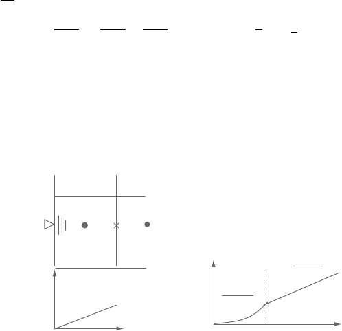
(a)
PNn
y
*
(b)
y*
y
c
*
m
t abmy*
Γ
t
aby *
Sc
t
∞
Sc
t
∞
a
c
y*
2
Figure 9.28. (a) Near surfacecellarrangement andthe eddy viscositydistribution,
(b) turbulent diffusivity distribution.

Sunden CH009.tex 25/8/2010 10: 57 Page 367
AWFs of turbulence for complex surface flow phenomena 367
reduces to µ
t
= αβµy
∗
as in Figure 9.28a since equation (91) leads to µ
t
∝ O(y).
On constant surface concentration conditions, the surface limiting behaviour of
concentration and its fluctuation are:
c = a
c
+ b
c
y + c
c
y
2
+···,c
= a
c
+ b
c
y + c
c
y
2
+··· (93)
When the turbulent concentration flux −ρ
vc is modelled as −ρvc = µ
t
∂c/∂y,
−ρ{
a
c
a
v
+(b
c
a
v
+a
c
b
v
)y+(a
c
c
v
+c
c
a
v
)y
2
+···}=µ
t
(b
c
+2c
c
y+···) (94)
Thus,
t
∝ O(y
0
). (In the case of non-surface-disturbance,
t
∝ O(y
2
) due to
a
v
=0and a
c
=0.)Inthe context of theeddy viscositymodels,the turbulent scalar
diffusivity
t
is modelled using a turbulent Schmidt number as
t
= µ
t
/(µSc
t
);
thus, with equation (92) one can rewrite this as:
t
= αβ max{0,(y
∗
− y
∗
v
)}/Sc
t
(95)
In order to satisfy the limiting behaviour of
t
near the surface, the limiting
behaviour of Sc
t
is required as O(y
−1
).Thus, Sc
t
is:
Sc
t
=
$
Sc
∞
t
/(y
∗
/y
∗
c
), 0 ≤ y
∗
≤ y
∗
c
Sc
∞
t
, y
∗
c
< y
∗
(96)
where Sc
∞
t
is a prescribed constant. This simple two-segment variation profile of
Sc
t
leads to the turbulent diffusivity distribution as in Figure 9.28b:
t
=
$
α
c
y
∗2
/Sc
∞
t
,0≤ y
∗
≤ y
∗
c
αβy
∗
/Sc
∞
t
, y
∗
c
< y
∗
(97)
for the case of non-surface disturbance where
t
∝ O(y
2
). The coefficient α
c
and
y
∗
c
have the relation α
c
= αβ/y
∗
c
for connecting the two segments. Then, with
the assumption that the rhs terms can be constant over the cell, the simplified
concentration equation in the surface adjacent cell:
∂
∂y
∗
µ
Sc
+ µ
t
∂
c
∂y
∗
=
ν
2
k
P
∂
∂x
(
ρU
c
)
@
AB C
C
C
(98)
can be easily integrated analytically to form the boundary conditions of the
concentration at the surface, namely the surface concentration flux:
q
s
=−
µ
Sc
d
c
dy
s
=−
k
1/2
p
ν
A
C
(99)
or the surface concentration:
c
s
= c
n
+
q
s
ScD
C
ρk
1/2
P
+
ScC
C
E
C
µ
(100)
Sunden CH009.tex 25/8/2010 10: 57 Page 368
368 Computational Fluid Dynamics and Heat Transfer
d
x
y
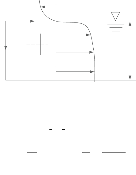
Air
Free surface
Computational domain
Water
Free slip
Figure 9.29. Computational domain of free-surface flows.
where the integration constants A
C
, D
C
and E
C
are
A
C
=
{
µ(c
n
− c
s
)/Sc +C
C
E
C
}
/D
C
(101)
D
C
=
1
α
1/2
cd
tan
−1
(α
1/2
cd
y
∗
c
) −
1
α
ct
ln
1 +α
ct
y
∗
c
1 +α
ct
y
∗
n
(102)
E
C
=
1
α
ct
(y
∗
c
− y
∗
n
) −
1
α
2
ct
ln
1 +α
ct
y
∗
c
1 +α
ct
y
∗
n
−
1
2α
cd
ln
1 +α
ct
y
∗
c
(103)
with α
ct
= αβSc/Sc
t
and α
cd
= α
ct
/y
∗
c
. The model coefficients are Sc
∞
t
=0.9,
β =0.55 and y
∗
c
=11.7.
Examples of applications
The example case is a fully developed counter-current air–water flow driven by a
constant pressure gradient. Figure 9.29 illustrates the coordinate system and the
computational domain applied in the present computations. Only the water phase
is solvedwith the non-disturbance and theconstantconcentration conditions at the
free surface.At the bottom of the domain, a free slip and a constant concentration-
flux condition are imposed. The coupled turbulence model for core flows is the
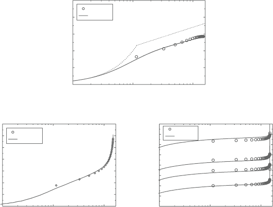
standardk-ε model.Figure9.30a–ccomparethepresentapplicationresultswiththe
DNS results of the free-surface turbulent flow with surface-shear whose Reynolds
number is Re
τ
=150 by Hasegawa and Kasagi [47]. Figure 9.30a shows that the
agreementbetweenthepresentandtheDNSresultsofthemeanvelocitydistribution
is satisfactory and the profiles are significantly lower than that of the log-law line
for wall turbulence. Figure 9.30b and c compare the mean concentration fields of
1 ≤ Sc ≤ 10
3
. The concentration profiles reasonably agree with the DNS results
in the various Schmidt numbers. This means that the AWF model can reproduce
essential near-surface behaviour of high Schmidt number turbulent flows.
Sunden CH009.tex 25/8/2010 10: 57 Page 369
AWFs of turbulence for complex surface flow phenomena 369
500
300
100
Sc =1,000
C
+
C
+
2 5
30
35
20
15
10
5
0
2 50
300
350
400
200
150
100
50
0
(b) (c)
1 10 100
y
+
1 10 100
y
+
Present
DN S
Present
DN S
(a)
2 5
20
15
U
+
U
+
=y
+
U
+
= 2.5 ln y
+
+ 5.5
10
5
0
1 10 100
y
+
Present
DN S
Figure 9.30. (a)Meanvelocitydistributionofaturbulentfree-shearboundarylayer,
(b) mean concentration distribution near a free surface at Sc=1,
(c) mean concentration distribution near a free surface at Sc=100–
1,000.
9.5 Conclusions
TheAWFs, whicharefor thereplacement oftheLWF andthetreatmentofcomplex
surfaceflowphenomena, havebeensummarised.Theiroverallstrategiesforderiva-
tionandimplementationhavebeenpresentedwithtypicalapplicationresults. From
the results,it has beenshown thattheAWFs arevalidin many important flows over
awiderange ofReynolds,PrandtlandSchmidtnumbers.Theeffectsofwallrough-
ness and/or wall permeability can be also included in the AWF as well. Although
they do not include the conventional log-laws, the AWFs accurately reproduce the
logarithmicprofiles of mean velocities and temperatures without grid dependency.
TheAWFs perform well with second moment closures, linear and nonlinear k − ε
models while the predictive accuracy depends on the turbulence model employed
inthe mainflow field.The computationalcostrequired fortheAWFsiscomparable
to that of the standard LWF.
Intherough-wallversionoftheAWF,theeffectsofwallroughnessonturbulence
and heat transfer are considered by employing functional forms of equivalent sand
grain roughness for the non-dimensional thickness of the modelled viscous sub-
layer and the turbulent Prandtl number immediately adjacent to the wall.
Sunden CH009.tex 25/8/2010 10: 57 Page 370
370 Computational Fluid Dynamics and Heat Transfer
Although the permeable-wall version of the AWF does not need to resolve
the region inside a permeable wall, by non-linearly linking to the solution of the
modified Brinkman equations for the flows inside porous media, it can bridge
the flows inside and outside of the porous media successfully. Since the com-
putedturbulentflowfieldsoverpermeableporoussurfacesarereasonably inaccord
with the corresponding data, theAWF for permeable wall turbulence models such
complicated wall-flow interactions.
By linking to the correct near-wall variation of turbulent viscosity µ
t
∝ y
3
,
the AWF can be successfully applicable to flows over a wide range of Prandtl
numbers up to Pr=4×10
4
, for smooth wall cases. (For flow fields and thermal
fields at Pr≤1, it is not totally necessary to employ the correct near-wall variation
ofturbulent viscosity.) Forrough wallcases, itis confirmed thatthemodel function
of Pr
t
inside roughness elements enables theAWF to perform well in high Pr flows
at least at Pr≤10.
With a slight modification, the AWF can reproduce the characteristics of the
turbulence near free surfaces.The predictive performance of such a version of the
AWF isreasonable inturbulent concentration fieldsin the rangeof Sc=1 to1,000.
Acknowledgements
The author thanks Professors B. E. Launder, H. Iacovides and Dr.T. J. Craft of the
Universityof Manchesterfortheirfruitfuldiscussions andcommentsontheAWFs.
AppendixA
The analytical integration of the momentum and energy equations (17) and (18) is
performed in the four different cases illustrated in figure 9.8. The process for the
case (a) y
v
< 0 is as follows:
The integration of equation (17) with equation (40) is:
If y
∗
≤ h
∗
,
dU
dy
∗
=
A
U
µ{1 +α(y
∗
− y
∗
v
)}
=
A
U
µY
∗
(A.1)
U =
A
U
αµ
lnY
∗
+ B
U
(A.2)
At a wall: y
∗
=0, the condition U =0 leads to:
B
U
=−
A
U
αµ
ln(1 − αy
∗
v
) =−
A
U
αµ
lnY
∗
w
(A.3)
When h
∗
< y
∗
, the integration leads to:
dU
dy
∗
=
C
U
y
∗
+ A
U
µY
∗
(A.4)
Sunden CH009.tex 25/8/2010 10: 57 Page 371
AWFs of turbulence for complex surface flow phenomena 371
Table 9.A1. Cell averaged generation P
k
, and integration constant: A
U
; (a) y
v
<
0, (b) 0 ≤ y
v
≤ h, (c) h ≤ y
v
≤ y
n
, (d) y
n
≤ y
v
; U
w
= 0 for
non-permeable walls
Case P
k
(a)
α
µ
2
y
∗
n
k
P
ν
=
&
h
∗
0
(y
∗
− y
∗
v
)
A
U
Y
∗
2
dy
∗
+
&
y
∗
n
h
∗
(y
∗
− y
∗
v
)
C
U
(y
∗
− h
∗
) +A
U
Y
∗
2
dy
∗
>
(b)
α
µ
2
y
∗
n
k
P
ν
=
&
h
∗
y
∗
v
(y
∗
− y
∗
v
)
A
U
Y
∗
2
dy
∗
+
&
y
∗
n
h
∗
(y
∗
− y
∗
v
)
C
U
(y
∗
− h
∗
) +A
U
Y
∗
2
dy
∗
>
(c)
α
µ
2
y
∗
n
k
P
ν
&
y
∗
n
y
∗
v
(y
∗
− y
∗
v
)
C
U
(y
∗
− h
∗
) +A
U
Y
∗
2
dy
∗
(d) 0
Case A
U
(a)
$
αµ(U
n
− U
w
) −C
U
(y
∗
n
− h
∗
) +C
U
Y
∗
w
α
+ h
∗
ln[Y
∗
n
/Y
∗
h
]
%
D
ln[Y
∗
n
/Y
∗
w
]
(b)
$
αµ(U
n
− U
w
) −C
U
(y
∗
n
− h
∗
) +C
U
Y
∗
w
α
+ h
∗
ln[Y
∗
n
/Y
∗
h
]
%
D
αy
∗
v
+ lnY
∗
n
(c)
$
αµ(U
n
− U
w
) −C
U
(y
∗
n
− y
∗
v
) +C
U
Y
∗
w
α
+ h
∗
lnY
∗
n
−
α
2
C
U
(y
∗2
v
− 2h
∗
y
∗
v
+ h
∗2
)
%
/
αy
∗
v
+ lnY
∗
n
(d)
$
µ(U
n
− U
w
) −
1
2
C
U
(y
∗2
n
− 2h
∗
y
∗
n
+ h
∗2
)
%
E
y
∗
n
U =
C
U
αµ
y
∗
+
A
U
αµ
−
Y
∗
w
C
U
α
2
µ
lnY
∗
+ B
U
(A.5)
Then, a monotonic distribution condition of dU/dy
∗
and U at y
∗
= h
∗
gives:
A
U
µY
∗
h
=
C
U
h
∗
+ A
U
µY
∗
h
(A.6)
A
U
αµ
lnY
∗
h
+ B
U
=
C
U
αµ
h
∗
+
A
U
αµ
−
Y
∗
w
C
U
α
2
µ
lnY
∗
h
+ B
U
(A.7)
Since at y
∗
=y
∗
n
the velocity is U = U
n
(U
n
is obtainable by interpolating the
calculated node values at P,N),
U
n
=
C
U
αµ
y
∗
n
+
A
U
αµ
−
Y
∗
w
C
U
α
2
µ
lnY
∗
n
+ B
U
(A.8)
TheintegrationconstantsA
U
, B
U
, A
U
andB
U
arethuseasilyobtainablebysolving
equations (A.3, A.6–A.8).

Sunden CH009.tex 25/8/2010 10: 57 Page 372
372 Computational Fluid Dynamics and Heat Transfer
Table 9.A2. Coefficients in equation (45)
Case D
T
(a)
−β
T
h
∗
α
T
− β
T
+
α
T
Y
βT
h
(α
T
− β
T
)
2
ln( Y
αT
h
/λ
b
) +
1
α
T
ln( Y
αT
n
/Y
αT
h
)
(b)
α
T
y
∗
v
− β
T
h
∗
α
T
− β
T
+
α
T
Y
βT
h
(α
T
− β
T
)
2
ln( Y
αT
h
/Y
βT
h
) +
1
α
T
ln( Y
αT
n
/Y
αT
h
)
(c)
1
α
T
lnY
αT
n
+ y
∗
v
(d) y
∗
n
Case E
T
(a)
h
∗
− y
∗
n
α
T
+
1
α
T
=
Y
αT
w
α
T
+ h
∗
−
Y
αT
h
α
T
− β
T
λ
b
β
T
α
T
− β
T
+ 1
+
λ
b
α
T
Y
βT
h
(α
T
− β
T
)
2
>
ln( Y
αT
n
/Y
αT
h
)
+
α
T
λ
b
Y
βT
h
(α
T
− β
T
)
3
ln( Y
αT
h
/λ
b
) −
h
∗
α
T
− β
T
1 +
β
T
h
∗
2
+
β
T
λ
b
α
T
− β
T
(b)
h
∗
− y
∗
n
α
T
+
1
α
T
=
Y
αT
w
α
T
+ h
∗
−
Y
αT
h
α
T
− β
T
λ
b
β
T
α
T
− β
T
+ 1
+
λ
b
α
T
Y
βT
h
(α
T
− β
T
)
2
>
ln( Y
αT
n
/Y
αT
h
)
+
α
T
λ
b
Y
βT
h
(α
T
− β
T
)
3
ln( Y
αT
h
/Y
βT
h
) −
h
∗
α
T
− β
T
1 +
β
T
h
∗
2
+
β
T
λ
b
α
T
− β
T
+
y
∗
v
α
T
− β
T
α
T
Y
βT
h
α
T
− β
T
−
α
T
y
∗
v
2
(c)
y
∗
v
− y
∗
n
α
T
− y
∗2
v
/2 +
Y
αT
w
α
2
T
lnY
αT
n
(d) −y
∗2
n
/2
In this case, the wall shear stress τ
w
is written as:
τ
w
= (µ + µ
t
)
dU
dy
y=0
= µY
∗
w
k
1/2
P
ν
dU
dy
∗
y
∗
=0
=
k
1/2
P
A
U
ν
(A.9)
whose resultant form is the same as equation (27) and can be calculated with A
U
.
Since the cell averaged production term
P
k
of the turbulence energy k is
written as:
P
k
=
1
y
n
=
&
h
0
ν
t
dU
dy
2
dy +
&
y
n
h
ν
t
dU
dy
2
dy
>
(A.10)
=
α
y
∗
n
k
P
ν
=
&
h
∗
0
(y
∗
− y
∗
v
)
dU
dy
∗
2
dy
∗
+
&
y
∗
n
h
∗
(y
∗
− y
∗
v
)
dU
dy
∗
2
dy
∗
>
it can be calculated by substituting dU/dy
∗
with equations (A.1) and (A.4).
As for the thermal field, when y
∗
≤ h
∗
, applying equations (41) and (42) to the
energy equation (18), one can lead to:
∂
∂y
∗
$
µ
Pr
+
αµ(y
∗
− y
∗
v
)
Pr
∞
t
+ C
0
(1 −y
∗
/h
∗
)
%
∂
∂y
∗
= C
T
(A.11)

Sunden CH009.tex 25/8/2010 10: 57 Page 373
AWFs of turbulence for complex surface flow phenomena 373
Its integration follows:
$
µ
Pr
+
αµ(y
∗
− y
∗
v
)
Pr
∞
t
+ C
0
(1 −y
∗
/h
∗
)
%
d
dy
∗
= C
T
y
∗
+ A
T
(A.12)
d
dy
∗
=
{1 +β
T
(h
∗
− y
∗
)}(C
T
y
∗
+ A
T
)
1 +α
T
(y
∗
− y
∗
v
) +β
T
(h
∗
− y
∗
)
Pr
µ
(A.13)
The further integration leads to:
=−
$
C
T
λ
b
β
T
(α
T
− β
T
)
2
−
C
T
(1 +β
T
h
∗
) +β
T
A
T
α
T
− β
T
%
Pr
µ
y
∗
+
PrC
T
β
T
2µ(α
T
− β
T
)
y
∗2
+
C
T
λ
2
b
β
T
(α
T
− β
T
)
3
−
λ
b
{C
T
(1 +β
T
h
∗
) +β
T
A
T
}
(α
T
− β
T
)
2
+
(1 +β
T
h
∗
)A
T
α
T
− β
T
Pr
µ
ln[(α
T
− β
T
)y
∗
+ λ
b
] +B
T
(A.14)
When y
∗
> h
∗
d
dy
∗
=
Pr(C
T
y
∗
+ A
T
)
µ{1 +α
T
(y
∗
− y
∗
v
)}
=
Pr(C
T
y
∗
+ A
T
)
µY
αT
(A.15)
=
PrC
T
µα
T
y
∗
+
Pr
µ
=
A
T
α
T
−
C
T
Y
αT
w
α
2
T
>
lnY
αT
+ B
T
(A.16)
The integration constants A
T
, B
T
, A
T
and B
T
are readily obtainable by equations
(A.13–A.16) imposing the boundary conditions ( |
y=0
=
w
, |
y=y
n
=
n
) and
a monotonic distribution condition of d /dy
∗
and at y
∗
= h
∗
as in the flow
field.
In the case of a constant wall temperature, the wall heat flux q
w
can be
calculated as:
q
w
=−ρc
p
ν
Pr
+
ν
t
Pr
t
k
1/2
P
ν
d
dy
∗
w
=−
ρc
p
k
1/2
P
µ
A
T
(A.17)
whose resultant form is the same as equation (28) and can be calculated with A
T
.
In the other cases (b)–(d), integration can be performed by the similar
manner.

Sunden CH009.tex 25/8/2010 10: 57 Page 374
374 Computational Fluid Dynamics and Heat Transfer
Appendix B
The integrals of the functions are:
&
1
θa
dy
∗
=
&
1
1 +
α
Pry
∗3
Pr
t
dy
∗
(B.1)
=
a
3
$
1
2
ln
(y
∗
+ a)
2
y
∗2
− ay
∗
+ a
2
+
√
3tan
−1
2y
∗
− a
a
√
3
%
&
y
∗
θa
dy
∗
=
&
y
∗
1 +
α
Pry
∗3
Pr
t
dy
∗
(B.2)
=
a
2
3
$
−
1
2
ln
(y
∗
+ a)
2
y
∗2
− ay
∗
+ a
2
+
√
3tan
−1
2y
∗
− a
a
√
3
%
&
1
θb
dy
∗
=
&
1
1 +
αPr(y
∗
− y
∗
v
)
Pr
t
dy
∗
=
1
α
θ
ln|1 + α
θ
(y
∗
− y
∗
v
)| (B.3)
&
y
∗
θb
dy
∗
=
&
y
∗
1 +
αPr(y
∗
− y
∗
v
)
Pr
t
dy
∗
(B.4)
=
y
∗
α
θ
−
1 −α
θ
y
∗
v
α
2
θ
ln|1 + α
θ
(y
∗
− y
∗
v
)|
&
1
θd
dy
∗
=
&
1
1 +
αPr(y
∗
− y
∗
v
)
Pr
∞
t
+ C
h
max(0,1− y
∗
/h
∗
)
dy
∗
=−
β
T
y
∗
α
T
− β
T
+
$
β
T
λ
b
(α
T
− β
T
)
2
+
1 +β
T
h
∗
α
T
− β
T
%
(B.5)
× ln|(α
T
− β
T
)y
∗
+ λ
b
|
&
y
∗
θd
dy
∗
=
&
y
∗
1 +
αPr(y
∗
− y
∗
v
)
Pr
∞
t
+ C
h
max(0,1− y
∗
/h
∗
)
dy
∗
=−
β
T
y
∗2
2(α
T
− β
T
)
+
$
β
T
λ
b
(α
T
− β
T
)
2
+
1 +β
T
h
∗
α
T
− β
T
%
y
∗
(B.6)
−
=
β
T
λ
2
b
(α
T
− β
T
)
3
+
λ
b
(1 +β
T
h
∗
)
(α
T
− β
T
)
2
>
× ln|(α
T
− β
T
)y
∗
+ λ
b
|

Sunden CH009.tex 25/8/2010 10: 57 Page 375
AWFs of turbulence for complex surface flow phenomena 375
where α
θ
= αPr/Pr
t
, α
T
= αPr/Pr
∞
t
, a = (α
Pr/Pr
t
)
−1/3
β
T
=
$
C
h
/(Pr
∞
t
h
∗
), for y ≤ h
0, for h < y
λ
b
=1 − β
T
h
∗
− αy
∗
v
. (Note that integration constants are neglected in the
results.)
&
1
θc
dy
∗
=
&
1
1 +
α
Pr(y
∗
+ δ
v
)
3
Pr
∞
t
+ C
h
max(0,1− y
∗
/h
∗
)
dy
∗
=
ζ
α
T
−
!
η
c
β
T
− (η
a
− η
b
)(1 +β
T
h
∗
) −
η
b
2
(1 +β
T
[h
∗
+ η
a
])
"
(y)
−
1 +β
T
(h
∗
+ η
a
)
2
ln|y
∗2
+ η
b
y
∗
+ η
c
|
+{1 + β
T
(h
∗
+ η
a
)}ln|y
∗
+ η
a
|
(B.7)
&
y
∗
θc
dy
∗
=
&
y
∗
1 +
α
Pr(y
∗
+ δ
v
)
3
Pr
∞
t
+ C
h
max(0,1− y
∗
/h
∗
)
dy
∗
=
ζ
α
T
!
η
c
(1 +β
T
[h
∗
+ η
a
]) −
η
b
2
(β
T
[η
a
η
b
− η
c
]
+η
a
[1 +β
T
h
∗
])
(y) +
1
2
{β
T
[η
a
η
b
− η
c
] (B.8)
+ η
a
(1 +β
T
h
∗
)}ln|y
∗2
+ η
b
y
∗
+ η
c
|
−η
a
{1 +β
T
(h
∗
+ η
a
)}ln|y
∗
+ η
a
|
where α
T
= α
Pr/Pr
∞
t
,
ξ =
⎧
⎪
⎨
⎪
⎩
(−q +
#
q
2
+ p
3
)
1/3
+ (−q −
#
q
2
+ p
3
)
1/3
,ifq
2
+ p
3
≥ 0,
2
√
−pcos
1
3
cos
−1
q
p
√
−p
,ifq
2
+ p
3
< 0,
(B.9)
p =−β
T
/(3α
T
), q ={1 +β
T
(h
∗
+ δ
v
)}/(2α
T
),
η
a
= δ
v
− ξ, η
b
= 2δ
v
+ ξ, η
c
= δ
2
v
+ δ
v
ξ + ξ
2
+ 3p, ζ = 1/{η
a
(η
a
− η
b
) +η
c
}