Ames W.F., Roger C. Nonlinear equations in the applied sciences. Volume 185
Подождите немного. Документ загружается.

210
A.
S.
Fokas

Hamiltonian Structure and Integrability
Benno Fuchssteiner
University
of
Paderborn
D
4790
Paderhorn
Germany
1
Iiitroductioii
Whenever
a
quantity, or
a
set of quantities, evolves with time then we call this
a
dynamical
system.
The evolution of tlie universe certainly is
a.
dyna.mical system, however
a
compli-
cated one. The la.ws of evolution which govern
such
a
system are called the dynamical
laws.
To
describe dyiianucal systcnis we
itsiially
make suita.ble approximations
in
the hope
of finding valid descriptions of their clia.racteristic quantities. But even after such approx-
imations we mostly cannot write down explicitly liow these quantities depend on time,
usually sucli
a
dependeiice is
niucli
to9con~plicat~ed to be cotuputed explicitly. Therefore we
commonly write
down
dynamical systcnis
in
their infinitesimal form.
Considering
a
dynainical system
in
its infinitesimal form has many advantages. The
principal one
is
that sucli
an
infiiiitcsiinal description is possible even in those caws where
a
global
description is not feasihlc at.
all.
Tecltnically speaking,
an
infinitesimal description
leads to
a
diffcrential equa.t,ion, which
in
many cases
has
nonlinear terms due to the interac-
tion between different quantit,ies.
To
find
sucli
a.
differential equation we only have to know
a
suitable set of dynamical laws. Ilowever. solving
such
a
nonlinear differential equation for
arhitrary sta.rting points (initial coritlitions) is often
a
ho~~eless endeavor.
Fortunately, the infinitesimal tlescriptioii sometimes gives an insight into the essential
structures for the dyna.mics of
t.hc
syst,eni, or
at
least into those parts of the dynamics which
ca.n he described locally.
Speaking from
a.n
abstract.
viewpoint the niain objects of our interest are equations
of the form
tit
=
1i(u)
(1.1)
where
I<(%)
is
a
vector
field
oii
sonie
inanifold
Af
a,nd
where
11
denotes the general point
on this manifold. Since we
do
not.
restrict tlie size of the dimension of the manifold
M
this equation still compriscs
a.11
abuntlance of possible
dyna.nucal
systems. For example
u,
could he the collection of all rclcvant~ data of an cconomy, tlien equation
(1.1)
describes
the evolution of that economy. if’ith rcgard to size of the manifold, this would be
a
rather
simple dynamical system since tlie nianifoltl certainly 1ia.s finite dimension whereas most
systems we consider la.ter
011
will
tlesrribe
syst,etns on infinite dimensional manifolds.
Most notions which we
use
in
the st,utly of equation
(1.1)
do
ha.ve
a.
very intuitive meaning.
For
example, we call equa.tion
(1.1)
a.
flow
on
tlie underlying manifold. Thus we imagine
that
a
point is flowing along its path
on
t,lie
manifold.
Such
a.
path is called an
orbit
of
the system. Since
J<(ti)
describes t.he cliange
in
the position of
u
for infinitesimal times,
Nonlinear Equations
in
the Applied Sciences
21
1
Copyright
0
1992
by
Academic Ress, Inc.
All
rights
of
reproduction
in
any
form
reserved.
ISBN
0-12-056752-0
212
Benno
Fuchssteiner
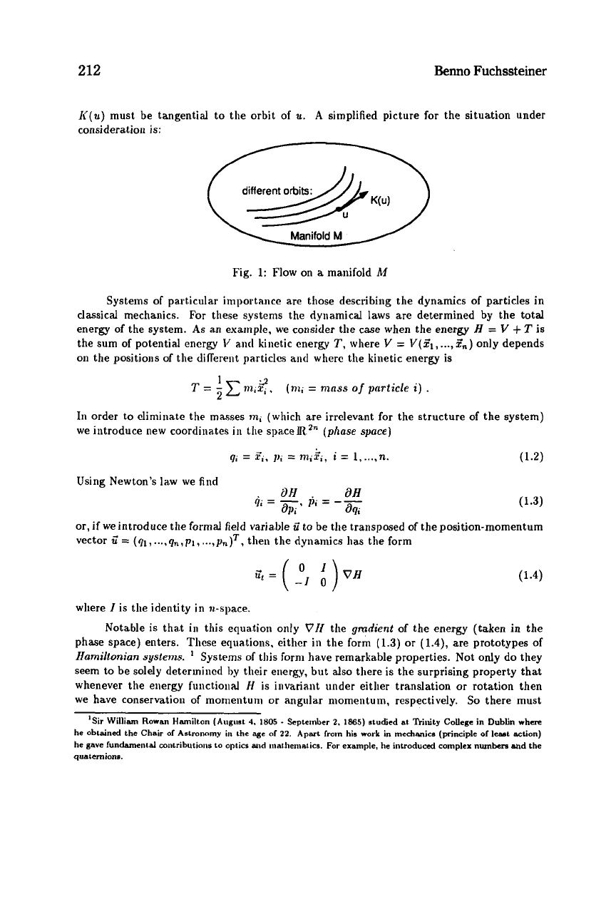
K(u)
must be tangential to the orbit of
u.
A
simplified picture
for
the situation under
consideration
is:
(
different
orbits:
Fig.
1:
Flow on
a
ma.nifold
A1
Systems
of
part,icular importance are those describing the dynamics of particles in
classical mechanics. For these systems the dynamical laws are determined by the total
energy
of
the system.
As
a.n example, we consider the case when the energy
H
=
V
+
T
is
the sum
of
potential energy
1'
and
kinet,ic energy
T,
where
V
=
I'(Z1,
...,
Zn)
only depends
on
the positions
of
the different particles and where the kinetic energy
is
1
9
T
=
-
wix,
,
2
(771,
=
nznss
of
pnrticle
i)
.
In
order to eliminate the mmses
n2,
(which are irrelevant for the structure
of
the system)
we introduce new coordinates
in
the spacem
2n
(phase space)
9,
=
?,,
IJ,
=
ni,.?,,
i
=
1
,...,
n.
(1.2)
Using Newton's law we find
BH
dH
q.
-
,
-
-,
1ji
=
--
hi
69i
or,
if we introduce the formal field varia.ble u'to be the transposed
of
the position-momentum
vector
u'
=
(a,
...,
qn,pl,
...,
pn)T,
then the dynamics
has
the form
where
I
is
the identity in n-space.
Notable
is
that
in
this equation only
VII
the
gmdient
of the energy (taken in the
phase space) enters. These equations, either
in
the form
(1.3)
or
(1.4),
are prototypes
of
Hamiltmian
systems. Systems
of
this form have remarkable properties. Not only do they
seem to be solely determined by their energy, but also there is the surprising property that
whenever the energy functional
fl
is invariant under either translation
or
rotation then
we have conservation
of
momentum
or
angular momentum, respectively.
So
there must
'Sir William Rowan
Hamilton
(August
4.
1805
-
September
2.
1865)
studied at 'hity College in Dublin where
he obtained the Chair
of
Astronomy in the age of
22.
Apart from his work in mechanics (principle
of
least action)
he gave fundamental contributions
to
optics and inatlieinat ics.
For
example. he introduced complex numben and the
quatemions.
Hamiltonian Structure
and
Integrability
213
be some kind
of
relation between tlie conservation laws
of
the system and its symmetry
structure. Indeed such
a
relation was revealed for cla.ssical IIamiltonian systems by Emmy
Noether' in her habilitation
[Is]
a.nd
this relation is nowadays generalized to symmetries
of
so-called Lie-Ba.cklund type for systems on infinite dimensional manifolds. The special
form of
(1.3)
or
(1.3)
is due to the special coordinate system which was chosen, whereas
the fundamental relation bet,weeii symmetries
and
conserved quantities certainly must go
beyond
a
structure which is the consequence
of
a
special coordinate system.
So,
in studying
Hamiltonian equations they must be analyzed in
a
differential geometric invariant setup such
that their structure becomes intlepentlcnt
of
special charts which were chosen to parametrize
the underlying manifold.
We
shall
do
that
in
the following sections
4
and
5.
The best known examples
of
Ilaniiltoiiian systems probably are the Harmonic Oscil-
lator and the nonlinear
peudiiliiiii,
drscrilwd I)elow:
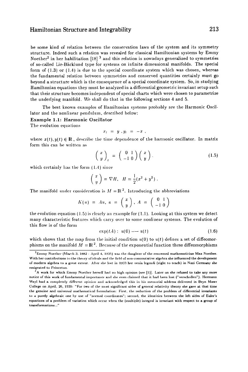
Example
1.1:
Harmonic
Oscillator
The evolution equations
.rt
=
y
.,I/(
=
--z
,
where
r(t),
g(t)
E
Ut
,
tlrscriI)e
tlit
t,iin('
tlrpciidriice
of
tlie harmonic oscillator.
In
matrix
form this ca.n
be
writtcii
RS
whiclr certainly
has
the
foriii
(1.4)
siiire
The inanifold
tiiider
coiisidrratioii
is
41
=
IIt
'.
Ii~trotlucing the abbreviations
(1.5)
the rvolution equation
(1
3)
is
dcady
iiii
csamplc
for
(1.1).
Looking at this system we detect
many characteristic features wliirli
carry
over
to
some
nonlinear systems. The evolution
of
this flow is
of
the forni
csp(1,l):
u(0)
--
u(t)
(1.6)
which shows that the
map
froiii
tlir
initial coiidition
~(0)
to
n(t)
defines a set
of
diffeomor-
phisms
on
tlie marlifold
Af
=
111
',
Hcc.;iuse
of the
espoiiential fuuction these diffeomorphisms
'Eninty Noether
(hlwc-li
3.
1882
-
April
4.
IlVJS)
was
the
rlaugliter
of
ihe
re~wwned
mathematician Max Noether.
With
her
contributions
tlir
thc,,ry
of
ideals
awl
11w
lickl
of
~~~,~~-Co~~~~~~~~tative algebra
she
influenced the development
01
modern algebra
to
a
grrat
eit~n.
After
SIIP
I~I
in
IYJ3
her wnia legendi (right
to
teach)
in
Nazi
Germany
she
emigrated
to
Princeton.
3A
work
for
which Emany
Noether
hersell
had
no
high
opinion
(see
[I)].
Later
on
she
refused
to take
any
more
notice
of
this work
of
fundamental
iniportaiwx
atid
die
even
claimed
that
it
had
Ixrn
lost
("verschollen").
Hcrmann
Weyl had
a
cnniplrtely diihcnt opinion
mid
arkn<wlrilgwi
tliis in his mcinwial address delivered
in
Bryn
Mawr
College
on
April,
26,
1935:
"For
two
of
tlic
tiicist
sigt"ficant sirlcs
of
general relativity theory she
gave
at
that
time
tlie
genuine
and
iuiiversal
mat
hema
tical f<,rmulation: First.
the
reduction
of
the
problem
01
differential invariants
lo
a
purely algebraic
one
by
use
of
''nnimal
coordinates";
second.
the
identities between the
left
sides of
Euler's
equations
01
a
problem of variation which occur
when
the
(multiple) integral is invariant with respect
to
a
group
01
transformat
ions
..."

214
Benno Fuchssteiner
form a represeiitatioii
of
the additive group
(111,
+).
Furthermore, we observe the advantage
of
introducing
polar
coortliiiiitcs
r
=
dm
and
9
=
arctan(y/z). Then in this new
coordinate space the system
I~econies
a
flow
with constant velocity dong the coordinate
lilies
I'
=
roridnnt.
Thus
iii
this
case
we
are
able
to split
up
tlie coordinates into two sets,
one set
(action vnricrbles)
wliich reiiiaiiis constant under tlie flow, and another set
(angle
ucrria6les)
wliicli
grows
on
the orlits linear with time.
If
sucli specid coordinates having
these properties can
Iw
introduced then we call
sucli
a
system
completely integrable.
Look-
ing
back
at
our
t~x~iiiplc
we
sw
that this notion
of
complete integrability must be related
to
tlie
existence
of
one-paranietcr symmetry groups. This is because changing one
of
the
coordinates
and
Iciiviiig
t
lie
ot
Iicrs
iiiicliangetl
inoves
orbits into orbits.
So
this movement
along
coordinate
linrs
constitut,es
a
syrittnefry
qrmip.
0
Example
1.2:
Pendulum
The time developniciit~
in
this
cast'
is
ptt
+
sin(9)
=
0
we
scc
that
(1.7)
is
of
the
I'oriii
(1.1)
The
manifold
under
consideratioil again is
Af
=
RZ.
In
contrast to
(1.5)
this equation
constitutes a nonlinear
flow.
Again the dynamics
1ia.s
the form
(1.4)
since
1
2
(
Si')j<'))
=
T//.
I/
=
1
-
cos(r/)
+
-pz
Altliougli this is
a
iioiilinriir
Ilo\c
it
ciin
Iw
lintwrized
locally
by introducing
a
suitable
coordinate
system.
Jlat this cooriliri;rte system
is
no
longer given by polar coordinates.
Obviously tlie
part.
of
tlie
coortlinatr
liiics
wliicli we called action variables should now be
given by the
lines
I/
=
roti..;/crii/
and
the
rcniaining part should
be
chosen in
a
suitable way.
IIow
to
do this
will
lie
desrrilw(l
1atc.r
on.
0
The
scope
of
this
art,icIc
is
to
rcplirasc~
tliesc
simple observations which we made
for
the liarinonic oscillator
in
a
gcwcriil
franicwork
so
that they can be carried over to other
more complicated system.
Fnrt
Iierinore,
we
want to formulate the corresponding notions
and relations
in
sucli
a way that tliry
arc
intlependeiit
of
the coordinate systems which we
choose.
We
organize
t.lic
art.iclr
in
the
following way:
In
tlie nest section, we introduce some
basic notions wliicli
lead
in
Scctioii
:$
to
a
description
of
the connection between symmetries
and coilserved qiiant.ities.
.4t
tliat point
we
shall
not yet choose the iiiost abstract setup
for
the descri1)t.iou.
Instcad
of'
foriiiiilatiiig evcrything
in
a
differential geometric invariant
way we still
will
work
with coordinate systems. This we do
in
order to keep the level
of
abstraction at tlic Iwginning
as
low
as
possi1)le. Results
in
these sections are mostly

Hamiltonian Structure and Integrability
215
presented without proofs because later on proofs will be given in
a
short and concise way
by using
a
higher level
of
abstraction.
In
Section
4
we introduce Lie algebra modules, Lie
derivatives and tensors in order to have
a
notation which allows one to see which notions
are geometrically invariant.
In
Section
5
we introduce the notion of bi-hamiltonian fields
on
a
general level. Then,
in
the following section, we introduce compatibility, especially
for hamiltonian pairs, and illustrate the power of this notion by
a
set
of
suitable examples
(Section
7).
In the
final
part, Section
8,
we discuss complete integrability in the finite
dimensional case and we show how that notion is connected to the situation considered
before. In addition the actionlangle structure
of
the multisoliton manifolds is given
2
Basic Notioiis in Chart Representation
I
hope that most readers a.re acquainted with notions like manifolds, vector fields, tangent
space, differentiability
and
so
on. However,
I
do not believe that a knowledge of the theo-
retical background
in
tnnnifoltl analysis is really necessary for understanding the concepts
described
in
this a.rticle. For the most part a. more intuitive grasp
of
infinitesimal calculus
and
a
heuristic idea
of
manifolds as being sometliing like smooth surfaces seems sufficient.
For the sake
of
coniplctciiess however. \ve include some remarks
on
this subject since
notation will differ somewhat from the conventional notation, insofar
as
we avoid the
cd-
culus
of
exterior forms.
For infinite dimensional manifolds we
sill
use the notion
of
Hadamard differentiability
[2G,]
127.1
This is a. fairly weak iiotion wliicli nevertheless ensures the validity
of
the chain
rule.
A
function
F
:
El
-
E2
between two 1inea.r spaces is said to be
Hadamard-
diflerentiable
at
11
E
El
if
there is
a
continuous linear map
L
:
El
-
Ez
such that
1
lini
-{F(u
t
cv)
-
F(u)
-
cL[v]}
=
0
<-a
f
uniformly
in
v
on each compact subset
of
El.
The
linear operator
L,
and its application
L[v]
to
v
are then denoted by
F’(u)
and
F’(u)[v],
respectively. Of course,
F’(u)[v]
is most
easily computed from the
direcfionol
derivntiue
of
F
F(u
t
(2)).
d
dc
)c=O
F”a]
=
F’(.,[Zl]
=
-
If not otherwise mentioned functions are usually assumed to be Fa-functions, i.e. infinitely
often differentiable.
If
the manifold is
a
vector space
M
=
E,
then vector fields are the continuous maps
11‘
:
E
-
E
assigning to each
ti
E
A4
$ome vector
I<(u)
E
E.
Again, we assume vector fields
’AU
linear spaces
E
are
hwinied
LO
be locally
convex
Hausdorff
topological vector spaces. Usually
we
do not
describe explicitly
the
topology on
E.
We
rather
inlroduce a
vector
space
E’
of
linear functionals
on
E.
which
separate points, and
we
assume lhat
E
is endowed
with
the
weakest locally convex topology such
that
the elements
of E’
arc continuour
(1.e.
the
weak tupology with respec1
to
E*).
Spaces
L(E1,
&)
of
linear maps
€1
-
€2
are
then
endowed with the weakest topologv given by
the
dual
pairs
El,
E;
and
€2,
E;,
i.e.
the weakest convex
topology
such
that
all
Linear Rinctionals
,i
on
L(E8,
Ez)
given by
L
-
p(L)
=
p(L(u))
with
p
E
€2’.
u
E
€1
are
continuous

216
Benno Fuchssteiner
to be
C".
Thus they constitute
a
Lie algebra with respect to the
commutator
defined by
a
[li,G](u)
=
-
{G(u
+
cI<(u))
-
Ii(u
+
eG(u))}
acl,=o
(2.3)
=
G'(it)[Ii(u)]
-
I<'(it)[G(u)].
This Lie algebra is referred to as the
vector
field
Lie
algebra
.
Recall that the definition
of
a.
Lie-algebra implies that the map
(Zi',G)
-+
[K,G]
is bilinear, antisymmetric
([I<,G]
=
-[G,I<])
and such that for
all
IC,G,L
the
Jacobi
identity
[[Ii,G],L]
+
[[&Ic],G]
+
[[G,L],Ic]
=
0
(2.4)
holds.
In
fact this identity is easily verified by using the cha.in rule
of
differentiation.
If the manifolds
A4
which we consider are
not
linear spaces, then derivatives are defined
in the usual way by parametrizing, or iuodeling, manifolds by linear spaces. Although in
most
of
our
examples the undcrlying manifold is
a
vector spxe we briefly illustrate that
procedure for the sake
of
complet.eness. Those readers who do not care for technicalities
should skip the following paragraphs
up
to
the introduction
of
conserved quantities.
Let
A4
be some Hausdorff topological space and
E
some linear space, then we call
A4
a
C"-manifold
if
there are given
an
open covering
{
U,la
E
some index set}
of
M
and
homeomorp hisins
po
:
U,
-
16,
l',
open susets
of
E
such that for all
u
and
0
the overlap map
pa
o
pi'
is
a
C"-map
Vo
n
pp(U,
n
Uo)
+
E.
These
p,
can be considered
to
be
local coordinates for the corresponding
U,.
The collection
of
these
(U,,p,)
is defined to be
an
atlas.
Such
an
at,las
allows transfer of all aspects
of
the
differential structure from
E
to
A{.
For example,
a
map
p
on
A4
is defined to be
C"
if
all
the
p
o
pi'
are
C".
Consider
IL
E
Al,
then
a
chart
around
u
is
a
homeomorphism
p
from
an open neighborl~ood
11
of
it
into tl!e model spa.ce
E
such that for all
a
the map
p
o
pi'
defined
on
pa(
U)
n
V,
is
Cm.
Now, the notion
of
tangent space is easily introduced. The
tangent space
TuA4
at the point
it
is represented by the model space together with
a
chart.
The formal definition has to be such that it does not depend
on
the special chart which is
chosen, hence it must be given by eqiiivalence cla.sses with respect to different charts.
So,
for fixed
u,
we consider pairs
(p,v)
consisting
of
a.
chart around
u
and
a
vector
v
in the
model space.
In
these
pairs
we introduce
an
equivalence rela.tion
(p,,q)
I
(p2,vz)
defined
by
(p2
op;')'(p~(u))[ul]
=
~2.
Tlieii
T,AJ
is defined
to
be the set of equivalence classes
endowed with the obvious topology inherited from the model space, and
TM
denotes the
collection
of
all these taugent spaces and is called the
tangent buiidle.
However, working
with these equivalence classes is not always very practical,
so
locally around
u,
we choose
common representatives by fixing some cha.rt
p
around
u
and representing the tangent spaces
of
the points around
u
jointly by
(p,
E).
Then
a
map
li
:
A4
+
TM
which assigns to each
u
E
M
some element
of
TuA4
is said
to
be
a
Coo-vector field
if
it is locally
C"
with respect
to such
a
comnion representation. Similarly, we define locally the
co-vector space
TZM
by
(p,
E')
instead, and
co-vector fields
to be suitable C"-maps from
M
into the
cotangent
bundle
(collection
of
all
TlA4.)
Of course, strictly speaking, elements of
TtM
are again
equivalence classes
as
before (only in the definit,ion a.bove. one has to replace the derivatives
Hamiltonian Structure
and
Integrability
217
by suitable adjoints in order to leave the application of
a
co-vector
to
a
tangent vector
invariant under coordinate changes). It should be observed that the choice
of
a
common
representation around some point
71
E
A4
is the same
as
choosing
a
particular chart in the
manifold given by the tangent bundle.
If the manifold under consideration is
a
linear space, then we do not really need
all
these constructions because we then model the manifold by itself and for simplicity we
choose the canonical chart given by the identity function on the model space. The validity
of
the requirements above then follows from the usual transformation formulas of differential
calculus. In this case the tangent spaces
T,Af
and cotangent spaces
T,’M
can be identified
with
E
and
E’,
respectively, and we are back in the situation
M
=
E
which we studied at
the beginning.
We have clioscn this formal approach to manifolds in order
to
indicate that differential
calculus on abstract nia.nifolds is indeed
an
easy task and that nevertheless for practical
computations it mostly is sufficient to do analysis
on
linear spaces.
To
proceed, we consider again
ut
=
A’
(u)
,
11
E
A4
,
A4
some manifold.
(1.1)
C”-maps from the manifold
A4
into the scalars (eitherm
or
CC
)
are called
scalarfields.
A
scalar field
I(u)
is said to be
a
conserved quantity for
(1.1)
if
I’(u)[Ii(u)]
=
O
(2.5)
for
all
u
E
M.
The reason why this name
lins
been chosen is obvious: Take an orbit
u(t)
of
(l.l),
then by the chain rule we find
-1(71(t))
d
=
I’(U(t))[I<(U(t)]
=
0.
dt
Hence, (2.5) guarantces that
I
is constant along the orbits
of
(1.1).
Observe that, for every
7~
E
Af,
the quantity
I’(u)
is
a
continuous linear functional on
the tangent space
T,A4,
i.e.
I’(u)
must be
a
cotangent vector. Derivatives
of
scalar fields
are called gradients and
f.
Therefore we use for scalar quantities
I
the notation
VI(u)
instead
of
Z’(u).
If
we write
<,
>
for the duality between tangent and cotangent vectors,
then
(2.5)
is writteii
as
<
VI,Ii
>
=
0.
(2.7)
Sometimes there is some advantage
iii
looking at conserved quantities which depend explic-
itly
on
time.
A
family
F(u,t)
of
scalar
fields depending in
a
Cm-way on the parameter
t
is
said to be
a
time dependent conserved quantity
if
F‘(u,t)
+
<
VF(u,t),I<(u)
>
=
0.
(2.8)
Here sub-t denotes partial derivative with respect to
t
and
V
F
=
F’
is taken by ignoring
the parameter
1.
The notion
makes
sense
because it gives
d
-F(~(t),t)
dt
=
0
(2.9)

218
Benno Fuchssteiner
which implies that
F(u(t),t)
is constant along the orbits of
(1.1).
From the physical point
of
view such
a
quantity does not seem to be very significant, since it is not invariant with
respect to
a
translation
of
time, Nevertheless it turns out that it
is
a
rather interesting
quantity from tlre computational point
of
view.
Of special interest are those conserved quantities which are linear in
t.
Let
F(u,l)
=
fo(u)
+
fi(U)t
(2.10)
fl
+
<Vfo,Ii>
=
0.
(2.11)
be such
a
quantity. Inserting
F
into
(2.8)
we then obtain by comparison
of
coefficients
Hence,
F(u,t)
is uniquely deternuned by its absolute term
fo(u).
Furthermore, the term
!I(.)
must be
a
conserved quantity which is time independent.
Related to conserved qnantities are one-parameter groups
of
C"-diffeomorphisms on
the manifold
M.
Recall that these are defined to be one-to-one C"-maps such that the
inverse is again differentiable.
A
one-parameter group
of diffeomorphisms is
a
map
(u,t)
-
R(T)(u) which is differentiable
on
the product
A4
xIR
=
{(u,~)Iu
E
M,r
EJR}
and assigns to every
T
E
IR
some diffeomorphism R(r)
:
M
-
A4
such that
R(r1
+r2)
=
f?(rl)oR(rz)
and
R(0)
=
I
(2.12)
for
all
TI,T~
E
IR
.
This implies that all the R(r) do commute and that R(-r) must be
the inverse
of
R(r). With other words:
R(T)
defines
a
group representation
of
the additive
group
(lR,
t).
One-parameter groups are completely determined by their r-derivative at
r
=
0.
To
see this let
R(T)
be a one-parameter group then
(2.13)
is said to be its
infinitesimnl
generator.
Equation
(2.13)
is an abbreviation for G(u)
=
(d/dr){R(r)(u)}lr=o. Since R(T) assigns to each point
of
the manifold another point, G
must assign to each manifold point
u
a
tangent vector at
u
.
Hence
G
is
a
vector field.
Because
of
the functiond equation
(2.12)
the r-derivative
of
R(T) at arbitrary
T
is easily
expressed by
G:
d
--R(T)
=
G"R(r).
dr
(2.14)
Hence R(T) is uniquely determined by the vector field G(u).
If the R(T) are linear then G again is linear. Then the solution of the linear differ-
ential equation
(2.14)
can formally be written as R(T)
=
exp(rG). In general however,
diffeomorphism groups are far from being groups
of
linear transformations. Nevertheless
their structure is more
or
less given by the exponential function since by use
of
pull-backs
equation
(2.14)
can be transformed
into
a linear differential equation (on some abstract
manifold with rather high dimension, however).
To
see this, consider
3
=
C"(AI,IR)
or c"(A4,C
),
respectively, the vector space
of scalar fields. Let R
:
A4
+
Af
be
a
C"-map then
(R'fNti)
:=
f(R(ti))
,
f
E
F
(2.15)
Hamiltonian Structure and Integrability
219
defines
a
map
R'
:
3
-
3
which is linear
on
3.
R'
is said to be the
pull-back
given by
R.
Similarly,
iE
1;
is
a
vector field we define
a
map
LI~
:
3
-+
3
(2.16)
by assigning to each
f
E
3
its derivative in the dir&tion
Ii.
Lr;
is said to be the
Lie-
derivative
given by
li.
Again, this is
a
linear map on
3
.
The space
of
all
Lie-derivatives is a vector space. The usual commutator of linear
(2.17)
maps
endows this vector spa.ce in
a
na.tural way with
a
Lie-algebra structure.
Observation
2.1:
of
vector fields
oiito
the
Lie-derivatives,
i.e.
we
have
[L,;, Lc]
=
L/iOLG
-
LGOLK
The map
A'
-
Lr; is a Lie-algebra isomorphism
from
the Lie algebm
L[/~,GI
=
[LI~, Lc]
(2.18)
for
all vector fields
1;
and
G.
The proof
is
simple. since by differentiation we see that the commutator bracket is
a
representation
of
the vector field bracket. Moreover, the required fact that
Lr;
#
Lc
whenever
1;
#
G
follows
from
the observation that for any two different tangent vectors
in
TuM
we can find
a
scalar
field
(by
application of
a
suitable co-vector) having different
derivatives in the direction
of
these tangent vectors. By similar arguments we find
Ri
#
R;
whenever
R1
#
Rz.
Hence, it suffices to study the pull-backs and the Lie-derivatives instead
of the original objects.
For
these new quantities equation (2.14) translates into
d
-R*(r)
=
Lr;F(r).
dr
(2.19)
which is clearly
a
linear differential equation since only linear operations are involved. There-
fore we write
R*(r)
=
esp(rLK)
(2.20)
thus obtaining
a
representation
of
the one-parameter group in terms of its infinitesimal
generator. Of course, this is
a
highly artificial representation, since
R'(r)
and
LK
act on
infinite-dimensional vector spaces even when
Af
is finite dimensional.
A
consequence of these considerations is that one-parameter groups and evolution
equations, whether linear
or
iionlinear, are more
or
less the same objects.
To
see
this, let
{&(r)lr
E
R}
be such
a
one-parameter
group
of diffeomorphisms
on
M
with infinitesimal
generator
G.
Since
G
is
a
vector field assigning
to
each
u
E
M
the tangent vector
G(u)
E
TuA4
we look at evolution equation
=
G(u).
(2.21)
In
fact, for a.ny initial condition
u(0)
a
solution is easily found, namely
741)
=
k(t)(u(O))
.
(2.22)