Armstrong M., et al. Plurigaussian simulations in geosciences
Подождите немного. Документ загружается.

Anisotropies
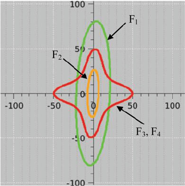
If the gaussian function model has a geometric anisotropy, the isovalue lines in the
variogram map are ellipses. Figure 6.7 shows the isovalue line for the indicator
variogram corresponding to 90% of the sill for the rocktype rule depicted in
Fig. 6.4. The two gaussian functions have exponential variograms with a geometric
anisotropy with ranges of 25 and 100. The long axis of continuity is oriented north-
southfor the firstgaussian function Z
1
,and east-westfor the othergaussian function
Z
2
. Th ese are independent.
For facies F
1
and F
2
, the isoline curves are still ellipses, as the truncation is
carried out on only one gaussian function. The shape is more complicated for facies
F
3
and F
4
(as they have the same proportions and are symmetrical in the rocktype
rule, their variograms are the same). The result looks like a combination of the two
ellipses in perpendicular directions.
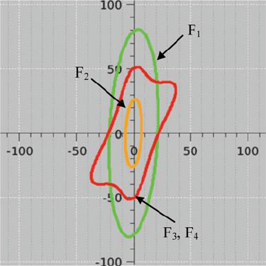
Figure 6.8 was obtained in the same way as Fig. 6.7 except that the anisotropy
axes have been rotated for Z
2
. The long axis is now north-east/south-west. We
immediately see that the isolines for facies F
1
and F
2
have not changed, as the
truncation for these facies is made only on Z
1
which has not changed. However, the
isolines for facies F
3
andF
4
havechanged markedly. Here the ellipses with both sets
of main anisotropy axes are superposed.
Fig. 6.7 For the facies of Fig. 6.4, isolines representing g(h) ¼ 90% of the sill. Long anisotropy
axes of the gaussian random functions are perpendicular
100 6 Variograms and Structural Analysis
Variogram Fitting
As the principle behind variogram fitting is the same in truncated gaussian case and
in plurigaussian case, both cases will be presented together.
Stationary Case
We now use the theoretical relation between the variograms of the underlying
gaussian variables and the facies indicators to fit models to them. We first choose a
modelforthegaussianfunction,tocalculatetheequivalentindicatormodelandtoplot
this. The key point in the variogram fitting is to have good quality experimental
variogramsinordertocomparethemwiththemodel.TheexamplesshowninFigs.6.7
and 6.8 show what is required (at least four directions are required to define the
variogram model in a given plane). If the data do not allow us to compute all these
experimentally, we need additional information, for example from the geologist.
In the plurigaussian case,if some faciesare defined by truncating on one gaussian
function only, it is better to fit them first. Once the values of the parameters for this
gaussianhavebeenfitted,thenthefaciesforthesecondgaussianfunctioncanbefitted.
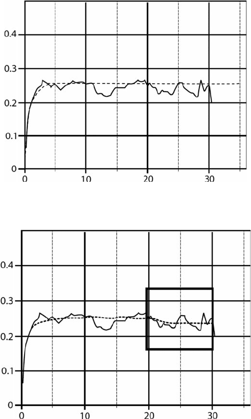
Figure 6.9 shows an example of fitting a vertical variogram in the stationary
case. Note that this vertical stationarity is not common. In this particular case,
experimental vertical proportions show a slight vertical non stationarity, which can
be interpreted as statistical fluctuations as there is no clear trend.
Fig. 6.8 For the facies of Fig. 6.4, isolines representing g(h) ¼ 90% of the sill. Long anisotropy
axes of the gaussian random functions make a 45
angle
Variogram Fitting 101
Non-stationary Case
The variogram fitting is done the same way as in the stationary case. We have to
average the theoretical variograms in the same way as the experimental variograms
(level by level or globally). In the non stationary case, the long distance variations
are completely controlled by the proportions. Figure 6.10 shows the same
Fig. 6.9 Example of stationary variogram fitting
Fig. 6.10 Example of use of the raw varying proportions in a stationary case
102 6 Variograms and Structural Analysis
experimental variogram as in Fig. 6.9, but the slight vertical non stationarity has
been taken into account during the fitting process.
Note that the long distances are better fitted here (see black square). Even in the
stationary case, it can be easier to fit the variogram with a non stationary approach
taking into account the experimental fluctuations of the proportions. The stationar y
proportions will be used for the simulation, together with the fitted variogram
model.Ifthe case isclearly non stationary,wecan choosetosmooth the proportions
Fig. 6.11 Non stationary variogram fitting using raw proportions
0.2
0.1
0
0102030
Vertical variogram
Nb. of steps
40 50
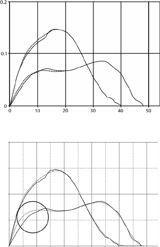
Fig. 6.12 Non stationary variogram computed using smoothed proportions
Variogram Fitting 103

for the simulation in order to reduce their experimental fluctuations, but the fitting
must be done with the raw proportions. Figure 6.11 shows a variogram fitting in a
non stationary case. Its shape is completely irregular, due to the marked variability
in the proportions. Figure 6.12 shows the variogram model obtained using the same
ranges but computed using smoothed proportions. Smoothing has produced quite
marked changes particularly near the origin. In some cases it has been impossible to
get a good fit after modifying the proportions. This difficulty can also appear when
using propor tions which vary in all directions. These proportions usually are the
result of estimation and do not come directly from a local average. There can be
higher discrepancies between the experimental “variograms” and the model curves.
A careful study of the proportions before the variogram fitting stage can reduce
these discrepancies.
Transition Probabilities
We saw earlier that transition probabilities are simple to compute whe n we know
the non-centred covariances of the indicator functions:
Pxþ h 2 F
j
x 2 F
i
j
¼
C
ij
x; x þ hðÞ
p
Fi
xðÞ
and
Pxþ h 2 F
j
x 2 F
i
and x þ h=2F
i
j
¼
C
ij
x; x þ hðÞ
p
Fi
xðÞC
ii
x;x þ hðÞ
These non centred covariances are easy to compute for the plurigaussian method:
C
ij
ðx,x þ hÞ¼
ðð
C
j
ðxþhÞ
ðð
C
i
ðxÞ
g
S
ðu
1
;u
2
;v
1
;v
2
Þdu
1
du
2
dv
1
dv
2
and
C
ii
ðx,x þ hÞ¼
ðð
C
i
ðxþhÞ
ðð
C
i
ðxÞ
g
S
ðu
1
;u
2
;v
1
;v
2
Þdu
1
du
2
dv
1
dv
2
This gives the following transition probabilities:
P½x þ h 2 F
j
x 2 F
i
j
¼
ÐÐ
C
j
ðxþhÞ
ÐÐ
C
i
ðxÞ
g
S
ðu
1
;u
2
;v
1
;v
2
Þdu
1
du
2
dv
1
dv
2
P
Fi
ðxÞ
and
P½xþh2F
j
x2F
i
j
andxþh=2F
i
¼
ÐÐ
C
j
ðxþhÞ
ÐÐ
C
i
ðxÞ
g
S
ðu
1
;u
2
;v
1
;v
2
Þdu
1
du
2
dv
1
dv
2
P
Fi
ðxÞ
ÐÐ
C
i
ðxþhÞ
ÐÐ
C
i
ðxÞ
g
S
ðu
1
;u
2
;v
1
;v
2
Þdu
1
du
2
dv
1
dv
2
104 6 Variograms and Structural Analysis

We see that these probabilities provide the same information as the non centred
covariances. They differ from variograms because they are not symmetrical in
general. For example, these probabilities are not symmetrical if the proportions
vary in the direction of the vector h, even if the gaussian functions have symmetri-
cal covariances:
ðð
C
j
ðxþhÞ
ðð
C
i
ðxÞ
g
S
ðu
1
;u
2
;v
1
;v
2
Þdu
1
du
2
dv
1
dv
2
6¼
ðð
C
i
ðxþhÞ
ðð
C
i
ðxÞ
g
S
ðu
1
;u
2
;v
1
;v
2
Þdu
1
du
2
dv
1
dv
2
These probabilities can also help to infer the value of the correlation r between the
gaussian functions, especially the second one:
P[x þ h 2 F
j
x 2 F
i
andx þ h =2 F
i
j¼
C
ij
ðx;x þ h Þ
P
Fi
ðxÞC
ii
ðx, x þ hÞ
Finally, they are easy to compute experimentally in the stationary case provided
that there are enough data points to be able to compute reliable statistics. For
example, we can only compute the second one when we have enough points within
the facies F
i
at level x, and enough points which are not in facies F
i
at level x + h.
Transition Probabilities 105
.
Chapter 7
Gibbs Sampler
Our ultimate objective is to simulate a gaussian random functi on with a specified
covariance structure, given the observed lithotypes (facies) at sample points. As the
lithotypes are known at these points, the correspo nding gaussian variables must
lie in certain intervals or sets but their values are not known. The difficulty is
that these random functions conditioned to the constraints are no longer gaussian
random functions.
InChap. 2, the two step procedure usedwas presentedfroma theoreticalpointof
view. Here we give a “maths-lite” presentation to illustrate the key concepts . The
first section presents several examples to explain why we have recourse to a Gibbs
sampler to gener ate gaussian values at sample points that have the right covariance
and belong to the right intervals. Once we have this set of point values, any method
for conditionally simulating gaussian random functions can be used; for example,
turning bands together with a conditioning kriging, sequential gaussian simula-
tions,LU decomposition,etc. See Chile
`
sand Delfiner (1999), Lantue
´
joul(2002a, b)
or Deutch and Journel (1992). As these techniques are well known, we will not
dwell on them here.
Why We Need a Two Step Simulation Procedure
The aim of thissection is to highlight the difficulties of simulating gaussian random
functions subject to interval constraints. To do this we consider three simple cases
where there are only two points:
l
With no constraint s
l
With interval constraints on one variable
l
With interval constraints on both variables
In the first case, the conditional distribution of Z(x) given Z(y) turns out to be
a gaussian distribution but this is no longer true in the other two cases. The con-
ditional distributions are merely proportional to gaussians.
M. Armstrong et al., Plurigaussian Simulations in Geosciences,
DOI 10.1007/978-3-642-19607-2_7,
#
Springer-Verlag Berlin Heidelberg 2011
107

Simulating Z(x) and Z(y) When There Are No Constraints
Consider two gaussian variables Z(x) and Z(y) with a correlation coefficient, r.In
order to simulate Z(x) given Z(y) we need to know its conditional distribution
which can be deduced from the joint distribution of the two variables:
gðu;v Þ¼
1
2p
ffiffiffiffiffiffiffiffiffiffiffiffiffi
1 r
2
p
exp
u
2
þ v
2
2ruvðÞ
2ð1 r
2
Þ
where u and v represent z(x) and z(y) respectively. This can be rewritten as
gðu,vÞ¼
1
s
ffiffiffiffiffiffi
2p
p
exp
u rvðÞ
2
2 s
2
()
1
ffiffiffiffiffiffi
2p
p
exp
v
2
2
(7.1)
where s
2
¼ 1 r
2
. The second term is just the marginal distribution of Z(y). The
first is the conditional distribution that we are looking for. It is clearly a gaussian
distribution with mean, rv, and variance s
2
. Equation (7.1) can be written as
gðu,vÞ¼g
v
(u)g(v) (7.2)
This is equivalent to the well-known decomposition:
ZðxÞ¼ rZðyÞþsRðxÞ
where R(x) is a N(0,1) residual that is independent of Z(y). If we estimate Z(x)
given z(y), the simple kriging weight equals r, and the SK variance is s
2
¼ 1 r
2
.
To simulate pairs of values of Z(x) and Z(y), we first draw two independent
N(0,1) values for Z(y) and R(x), then we substitute them into the decomposition
formula to get Z(x). Alternatively we could say that we draw one realisation v of
a N(0,1) variable for Z(y), followed a N(rv,s
2
) variable for Z(x). In that case, we
use the marginal distribution of Z(y) to draw a realisation of it, then the conditional
distribution of Z(x) given Z(y) to draw the other value directly. This is only possible
because the form of the conditional distribut ion is so simpl e.
Simulating Z(x) and Z(y) When Z(y) Belongs to an Interval
In this case Z(y) is known to lie in a specified interval, I, and we want to simulate
the pair of variables, Z(x) and Z(y), given that Z(y) lies in that interval. The joint
density of the two variables is now
hðu;v Þ¼kgðu;vÞ1
I
ðvÞ
108 7 Gibbs Sampler

where 1
I
ðvÞ is the indicator function for the interval I and k is the normation factor
required to ensure that the integral of h(u,v) sums to 1. So the joint density is
hðu;v Þ¼
1
s
ffiffiffiffiffiffi
2p
p
exp
1
2
u rvðÞ
2
s
2
()
k
ffiffiffiffiffiffi
2p
p
exp
1
2
v
2
1
I
ðvÞ
This can be written as
hðu;v Þ¼h
V
ðuÞ hðvÞ
It is clear that h(v) is the marginal distribution of a gaussian variable Z(y) restricted
to the interval I. To show that it is the marginal distribution, we just have to prove
that
ð
<
h
v
ðuÞdu = 1
Integrating h(u, v) with respect to u gives
ð
<
hðu;v Þ du ¼
ð
<
1
s
ffiffiffiffiffiffi
2p
p
exp
u rvðÞ
2
2s
2
()
du
k
ffiffiffiffiffiffi
2p
p
exp
v
2
2
1
I
ðvÞ
As the first term on the right hand side is just the integral of a N(rv,s
2
) variable, it
equals 1, which gives us the required result. In order to simulate these we use the
same interpretation as before: first simulate Z(y) in the interval I then simulate Z(x)
given that Z(y) 2 I. The first simulation is just a truncated gaussian; the second one
corresponds to simulating an independent N(rv,s
2
) variable. That is, we are still
using the classical decomposition.
But there is a fundamental change in the marginal distribution of Z(x). To
see this, we integrate the joint density with respect to v using (7.2) written as
gðu;v Þ¼g
u
ðvÞgðuÞ:
ð
<
hðu;v Þ dv ¼
ð
<
kgðu;vÞ 1
I
ðvÞ dv
¼
ð
<
1
s
ffiffiffiffiffiffi
2p
p
1
I
ðvÞ exp
ðv ruÞ
2
2s
2
()
dv
k
ffiffiffiffiffiffi
2p
p
exp
u
2
2
Ifwe lett ¼ v ru, thenv 2 I , t 2 I ru andthefirsttermon theright becomes
ð
<
1
s
ffiffiffiffiffiffi
2p
p
1
Iru
ðt) exp
t
2
2s
2
dt ¼ E1
Iru
Why We Need a Two Step Simulation Procedure 109