Articolo G.A. Partial Differential Equations and Boundary Value Problems with Maple V
Подождите немного. Документ загружается.

228 Chapter 4
10 20
220
215
210
25
0
515
Figure 4.1
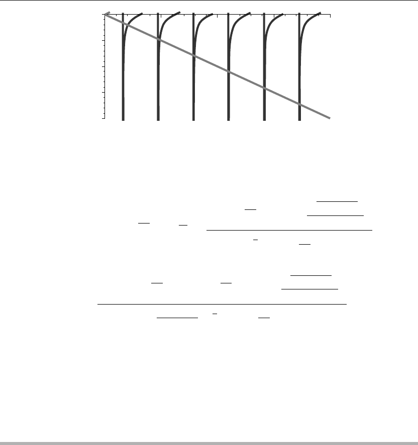
Combining all of the preceding, the final series solution to the problem reads
u(x, t) =
∞
n=1
2 sin
λ
n
x
e
−
t
10
⎛
⎜
⎜
⎜
⎝
−
4
cos
√
λ
n
−1
cos
√
25 λ
n
−4 t
20
3λ
3
2
n
cos
√
λ
n
2
+1
−
8
15 cos
√
λ
n
λ
n
+cos
√
λ
n
−1
sin
√
25 λ
n
−4 t
20
3
√
25 λ
n
−4 λ
3
2
n
cos
√
λ
n
2
+1
⎞
⎟
⎟
⎟
⎠
The detailed development of the solution of this problem and the graphics are given in one of
the Maple worksheet examples.
4.6 Example Wave Equation Problems in Rectangular
Coordinates
We now consider several examples of partial differential equations for wave phenomena under
various homogeneous boundary conditions over finite intervals in the rectangular coordinate
system. We note that all of the spatial ordinary differential equations in the rectangular
coordinate system are of the Euler type; thus, the weight function w(x) = 1.
EXAMPLE 4.6.1: We seek the wave distribution u(x, t) for transverse waves on a taut string,
over the finite interval I ={x |0 <x<1}. The string is tied at both ends. It is vibrating in a
viscous medium with small damping, and there are no external forces acting. The string has an
initial displacement distribution f(x) and an initial speed distribution g(x) given following.
The wave speed is c = 1/4, and the damping factor is γ = 1/5.

The Wave Partial Differential Equation 229
SOLUTION: The homogeneous wave equation is
∂
2
∂t
2
u(x, t) = c
2
∂
2
∂x
2
u(x, t)
−γ
∂
∂t
u(x, t)
The boundary conditions are type 1 at x = 0 and type 1 at x = 1
u(0,t)= 0 and u(1,t)= 0
The initial conditions are
u(x, 0) = x(1 −x) and u
t
(x, 0) = x(1 −x)
The ordinary differential equations from the method of separation of variables are
d
2
dt
2
T(t) +γ
d
dt
T(t)
+c
2
λT(t) = 0
and
d
2
dx
2
X(x)+λX(x) = 0 (4.2)
The boundary conditions on the spatial equation are
X(0) = 0 and X(1) = 0
Assignment of system parameters
> restart:with(plots):a:=0:b:=1:c:=1/4:unprotect(gamma):gamma:=1/5:
Allowed eigenvalues and orthonormal eigenfunctions are obtained from Example 2.5.1.
> lambda[n]:=(n*Pi/b)ˆ2;
λ
n
:= n
2
π
2
(4.3)
for n = 1, 2, 3,....
> X[n](x):=sqrt(2/b)*sin(n*Pi/b*x);X[m](x):=subs(n=m,X[n](x)):
X
n
(x) :=
√
2 sin(nπx) (4.4)
Statement of orthonormality with respect to the weight function w(x) = 1
> w(x):=1:Int(X[n](x)*X[m](x)*w(x),x=a...b)=delta(n,m);
1
0
2 sin(nπx) sin(mπx) dx = δ(n, m) (4.5)

230 Chapter 4
Time-dependent solution
> T[n](t):=exp((−gamma/2)*t)*(A(n)*cos(omega[n]*t)+B(n)*sin(omega[n]*t));
T
n
(t) := e
−
1
10
t
(A(n) cos(ω
n
t) +B(n) sin(ω
n
t)) (4.6)
Generalized series terms
> u[n](x,t):=T[n](t)*X[n](x):
Eigenfunction expansion
> u(x,t):=Sum(u[n](x,t),n=1..infinity);
u(x, t) :=
∞
n=1
e
−
1
10
t
(A(n) cos(ω
n
t) +B(n) sin(ω
n
t))
√
2 sin(nπx) (4.7)
> omega[n]:=sqrt(lambda[n]*cˆ2−gammaˆ2/4);
ω
n
:=
1
20
25 n
2
π
2
−4 (4.8)
From Section 4.5, the coefficients A(n) and B(n) are to be determined from the inner product of
the eigenfunctions and the given initial condition functions u(x, 0) = f(x) and u
t
(x, 0) = g(x).
> f(x):=x*(1−x);
f(x) := x(1 −x) (4.9)
> g(x):=x*(1−x);
g(x) := x(1 −x) (4.10)
For n = 1, 2, 3,...,
> A(n):=Int(f(x)*X[n](x)*w(x),x=a..b);A(n):=expand(value(%)):
A(n) :=
1
0
x(1 −x)
√
2 sin(nπx) dx (4.11)
> A(n):=simplify(subs({sin(n*Pi)=0,cos(n*Pi)=(−1)ˆn},A(n)));
A(n) := −
2
√
2(−1 +(−1)
n
)
π
3
n
3
(4.12)

The Wave Partial Differential Equation 231
> B(n):=Int((f(x)*gamma/2+g(x))*X[n](x)*w(x), x=a..b)/omega[n];B(n):=expand(value(%)):
B(n) :=
20
⎛
⎝
1
0
11
10
x(1 −x)
√
2 sin(nπx)dx
⎞
⎠
25n
2
π
2
−4
(4.13)
> B(n):=radsimp(subs({sin(n*Pi)=0, cos(n*Pi)=(−1)ˆn},%));
B(n) := −
44
√
2(−1 +(−1)
n
)
π
3
n
3
25n
2
π
2
−4
(4.14)
> T[n](t):=exp((−gamma/2)*t)*(A(n)*cos(omega[n]*t)+B(n)*sin(omega[n]*t)):
Generalized series terms
> u[n](x,t):=eval(T[n](t)*X[n](x)):
Series solution
> u(x,t):=Sum(u[n](x,t),n=1..infinity);
u(x, t) :=
∞
n=1
e
−
1
10
t
⎛
⎝
−
2
√
2(−1 +(−1)
n
) cos
1
20
25n
2
π
2
−4 t
π
3
n
3
(4.15)
−
44
√
2(−1 +(−1)
n
) sin
1
20
25n
2
π
2
−4 t
π
3
n
3
25n
2
π
2
−4
⎞
⎠
√
2 sin(nπx)
First few terms of sum
> u(x,t):=sum(u[n](x,t),n=1..3):
ANIMATION
> animate(u(x,t),x=a..b,t=0..20,thickness=3);
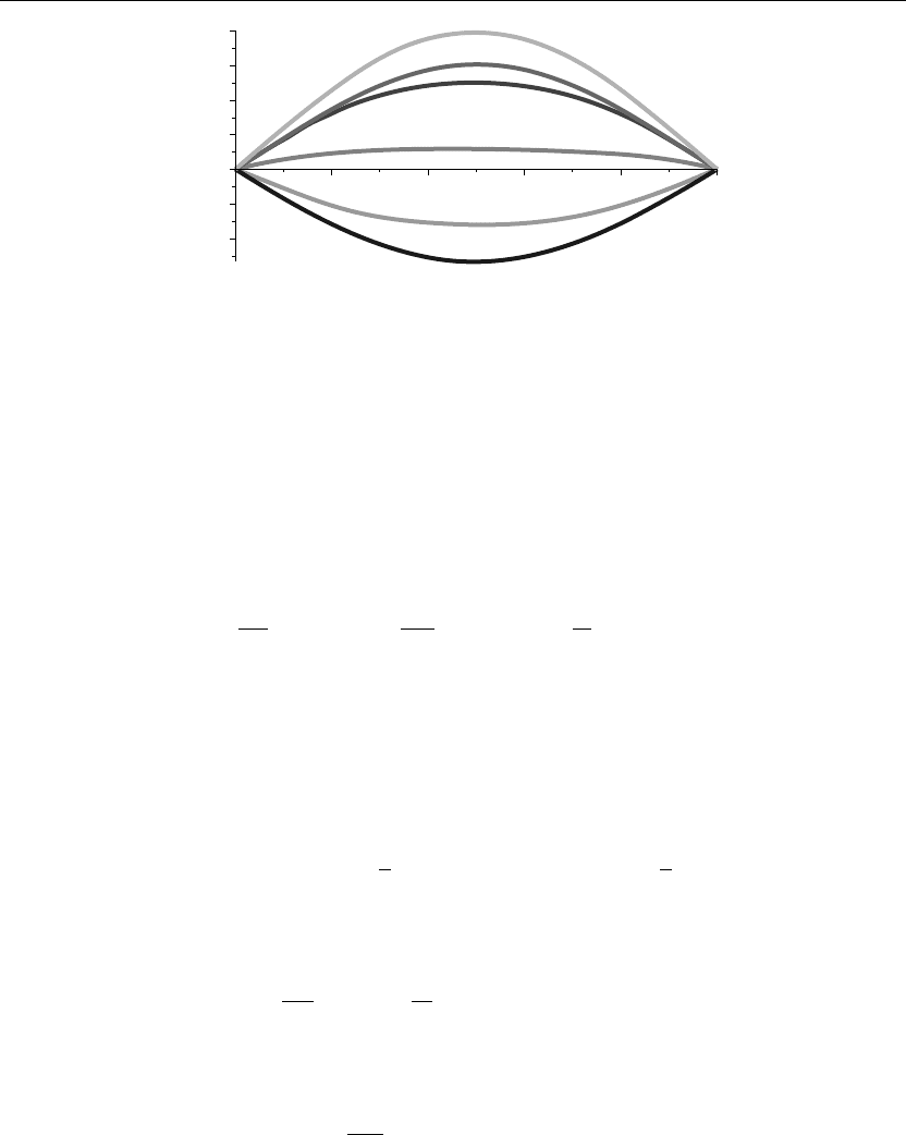
The preceding animation command illustrates the spatial-time-dependent solution for u(x, t).
The following animation sequence in Figure 4.2 shows snapshots of the animation at times
t = 0, 1, 2, 3, 4, and 5.
ANIMATION SEQUENCE
> u(x,0):=subs(t=0,u(x,t)):u(x,1):=subs(t=1,u(x,t)):
> u(x,2):=subs(t=2,u(x,t)):u(x,3):=subs(t=3,u(x,t)):
> u(x,4):=subs(t=4,u(x,t)):u(x,5):=subs(t=5,u(x,t)):
> plot({u(x,0),u(x,1),u(x,2),u(x,3),u(x,4),u(x,5)},x=a..b,thickness=10);
232 Chapter 4
x
0.2 0.4 0.6 0.8 1
20.2
20.1
0
0.1
0.2
0.3
0.4
Figure 4.2
EXAMPLE 4.6.2: We seek the wave distribution u(x, t) for longitudinal vibrations in a rigid
bar over the finite interval I ={x |0 <x<1}. The left end of the bar is secured, and the right
end is unsecured. The damping is very small, and the bar has an initial displacement
distribution f(x) and an initial speed distribution g(x) given as follows. The wave speed is
c = 1/4, and the damping factor is γ = 1/5.
SOLUTION: The homogeneous wave equation is
∂
2
∂t
2
u(x, t) = c
2
∂
2
∂x
2
u(x, t)
−γ
∂
∂t
u(x, t)
The boundary conditions are type 1 at x = 0 and type 2 at x = 1
u(0,t)= 0 and u
x
(1,t)= 0
The initial conditions are
u(x, 0) = x
1 −
x
2
and u
t
(x, 0) = x
1 −
x
2
The ordinary differential equations from the method of separation of variables are
d
2
dt
2
T(t) +γ
d
dt
T(t)
+c
2
λT(t) = 0
and
d
2
dx
2
X(x)+λX(x) = 0 (4.16)
The boundary conditions on the spatial equation are
X( 0) = 0 and X
x
(1) = 0

The Wave Partial Differential Equation 233
Assignment of system parameters
> restart:with(plots):a:=0:b:=1:c:=1/4:unprotect(gamma):gamma:=1/5:
Allowed eigenvalues and orthonormal eigenfunctions are obtained from Example 2.5.2.
> lambda[n]:=((2*n−1)*Pi/(2*b))ˆ2;
λ
n
:=
1
4
(2 n −1)
2
π
2
(4.17)
for n = 1, 2, 3,....
> X[n](x):=sqrt(2/b)*sin((2*n−1)*Pi/(2*b)*x);X[m](x):=subs(n=m,X[n](x)):
X
n
(x) :=
√
2 sin
1
2
(2n −1)πx
(4.18)
Statement of orthonormality with respect to the weight function w(x) = 1
> w(x):=1:Int(X[n](x)*X[m](x)*w(x),x=a..b)=delta(n,m);
1
0
2 sin
1
2
(2n −1)πx
sin
1
2
(2m −1)πx
dx = δ(n, m) (4.19)
Time-dependent solution
> T[n](t):=exp((−gamma/2)*t)*(A(n)*cos(omega[n]*t)+B(n)*sin(omega[n]*t));u[n](x,t):=
T[n](t)*X[n](x):
T
n
(t) := e
−
1
10
t
(
A(n) cos(ω
n
t) +B(n) sin(ω
n
t)
)
(4.20)
Generalized series terms
> u[n](x,t):=T[n](t)*X[n](x):
Eigenfunction expansion
> u(x,t):=Sum(u[n](x,t),n=1..infinity);
u(x, t) :=
∞
n=1
e
−
1
10
t
(
A(n) cos(ω
n
t) +B(n) sin(ω
n
t)
)
√
2 sin
1
2
(2n −1)πx
(4.21)
> omega[n]:=sqrt(lambda[n]*cˆ2−gammaˆ2/4);
ω
n
:=
1
40
25(2n −1)
2
π
2
−16 (4.22)
From Section 4.5, the coefficients A(n) and B(n) are to be determined from the inner product
of the eigenfunctions and the initial condition functions u(x, 0) = f(x) and u
t
(x, 0) = g(x).
234 Chapter 4
> f(x):=x*(1−x/2);
f(x) := x
1 −
1
2
x
(4.23)
> g(x):=x*(1−x/2);
g(x) := x
1 −
1
2
x
(4.24)
For n = 1, 2, 3,...,
> A(n):=Int(f(x)*X[n](x)*w(x),x=a..b);A(n):=(value(%)):
A(n) :=
1
0
x
1 −
1
2
x
√
2 sin
1
2
(2n −1)πx
dx (4.25)
> A(n):=factor(subs({sin(n*Pi)=0,cos(n*Pi)=(−1)ˆn},A(n)));
A(n) :=
8
√
2
(2n −1)
3
π
3
(4.26)
> B(n):=Int((f(x)*gamma/2+g(x))*X[n](x)*w(x),x=a..b)/omega[n];B(n):=(value(%)):
B(n) :=
40
1
0
11
10
x
1 −
1
2
x
√
2 sin
1
2
(2n −1)πx
dx
25(2n −1)
2
π
2
−16
(4.27)
> B(n):=subs({sin(n*Pi)=0,cos(n*Pi)=(−1)ˆn},B(n));
B(n) :=
352
√
2
π
3
(8n
3
−12n
2
+6n −1)
25(2n −1)
2
π
2
−16
(4.28)
Generalized series terms
> u[n](x,t):=eval(T[n](t)*X[n](x)):
Series solution
> u(x,t):=Sum(u[n](x,t),n=1..infinity);
u(x, t) :=
∞
n=1
e
−
1
10
t
⎛
⎝
8
√
2 cos
1
40
25(2n −1)
2
π
2
−16 t
(2n −1)
3
π
3
(4.29)
+
352
√
2 sin
1
40
25(2n −1)
2
π
2
−16 t
π
3
(8n
3
−12n
2
+6n −1)
25(2n −1)
2
π
2
−16
⎞
⎠
√
2 sin
1
2
(2n −1)πx
The Wave Partial Differential Equation 235
First few terms of sum
> u(x,t):=sum(u[n](x,t),n=1..3):
ANIMATION
> animate(u(x,t),x=a..b,t=0..20,thickness=3);
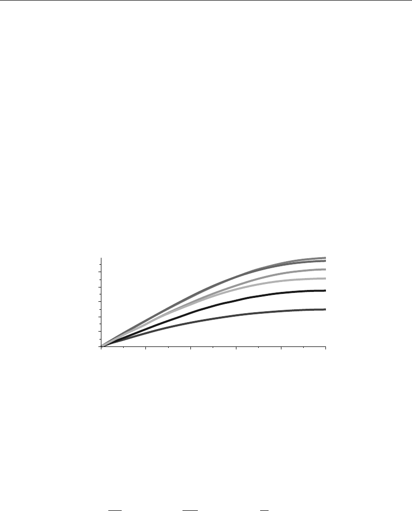
The preceding animation command illustrates the spatial-time-dependent solution for u(x, t).
The following animation sequence in Figure 4.3 shows snapshots of the animation at times
t = 0, 1, 2, 3, 4, and 5.
ANIMATION SEQUENCE
> u(x,0):=subs(t=0,u(x,t)):u(x,1):=subs(t=1,u(x,t)):
> u(x,2):=subs(t=2,u(x,t)):u(x,3):=subs(t=3,u(x,t)):
> u(x,4):=subs(t=4,u(x,t)):u(x,5):=subs(t=5,u(x,t)):
> plot({u(x,0),u(x,1),u(x,2),u(x,3),u(x,4),u(x,5)},x=a..b,thickness=10);
x
0 0.2 0.4 0.6 0.8 1
0
0.2
0.4
0.6
0.8
1.0
Figure 4.3
EXAMPLE 4.6.3: We again consider the waves describing the longitudinal vibrations in a
rigid bar over the finite interval I ={x |0 <x<1} with both ends unsecured. The damping is
very small. The initial displacement distribution f(x) and the initial speed distribution g(x) are
given following. The wave speed is c = 1/4, and the damping factor is γ = 1/5.
SOLUTION: The homogeneous wave equation is
∂
2
∂t
2
u(x, t) = c
2
∂
2
∂x
2
u(x, t)
−γ
∂
∂t
u(x, t)
The boundary conditions are type 2 at x = 0 and type 2 at x = 1
u
x
(0,t)= 0 and u
x
(1,t)= 0

236 Chapter 4
The initial conditions are
u(x, 0) = 4x
3
−6x
2
+1 and u
t
(x, 0) = 0
The ordinary differential equations from the method of separation of variables are
d
2
dt
2
T(t) +γ
d
dt
T(t)
+c
2
λT(t) = 0
and
d
2
dx
2
X(x)+λX(x) = 0 (4.30)
The boundary conditions on the spatial equation are
X
x
(0) = 0 and X
x
(1) = 0
Assignment of system parameters
> restart:with(plots):a:=0:b:=1:c:=1/4:unprotect(gamma):gamma:=1/5:
Allowed eigenvalues and orthonormal eigenfunctions are obtained from Example 2.5.4.
For n = 0,
> lambda[0]:=0;
λ
0
:= 0 (4.31)
> X[0](x):=1/sqrt(b);
X
0
(x) := 1 (4.32)
For n = 1, 2, 3,...,
> lambda[n]:=(n*Pi/b)ˆ2;
λ
n
:= n
2
π
2
(4.33)
> X[n](x):=sqrt(2/b)*cos(n*Pi/b*x);X[m](x):=subs(n=m,X[n](x)):
X
n
(x) :=
√
2 cos(nπx) (4.34)
Statement of orthonormality with respect to the weight function w(x) = 1
> w(x):=1:Int(X[n](x)*X[m](x)*w(x),x=a..b)=delta(n,m);
1
0
2 cos(nπx) cos(mπx) dx = δ(n, m) (4.35)

The Wave Partial Differential Equation 237
Time-dependent solution
> T[0](t):=A(0)+B(0)*exp(−gamma*t);
T
0
(t) := A(0) +B(0)e
−
1
5
t
(4.36)
For n = 0,
> T[n](t):=exp((−gamma/2)*t)*(A(n)*cos(omega[n]*t)+B(n)*sin(omega[n]*t));
T
n
(t) := e
−
1
10
t
(
A(n) cos
(
ω
n
t
)
+B(n) sin
(
ω
n
t
))
(4.37)
For n = 1, 2, 3,...,
Generalized series terms
> u[0](x,t):=T[0](t)*X[0](x):u[n](x,t):=T[n](t)*X[n](x):
Eigenfunction expansion
> u(x,t):=u[0](x,t)+Sum(u[n](x,t),n=1..infinity);
u(x, t) := A(0) +B(0)e
−
1
5
t
+
∞
n=1
e
−
1
10
t
(
A(n) cos
(
ω
n
t
)
+B(n) sin
(
ω
n
t
))
√
2 cos(nπx) (4.38)
> omega[n]:=sqrt(lambda[n]*cˆ2−gammaˆ2/4);
ω
n
:=
1
20
25n
2
π
2
−4 (4.39)
From Section 4.5, the coefficients A(n) and B(n) are to be determined from the inner product
of the eigenfunctions and the initial condition functions u(x, 0) = f(x) and u
t
(x, 0) = g(x).
> f(x):=4*xˆ3−6*xˆ2+1;
f(x) := 4x
3
−6x
2
+1 (4.40)
> g(x):=0;
g(x) := 0 (4.41)
For n = 0,
> A(0):=(Int((f(x)*gamma+g(x))/gamma*X[0](x)*w(x),x=a..b));
A(0) :=
1
0
(4x
3
−6x
2
+1) dx (4.42)