Bayro-Corrochano E., Scheuermann G. Geometric Algebra Computing: in Engineering and Computer Science

Подождите немного. Документ загружается.

308 D. Gonzalez-Aguirre et al.

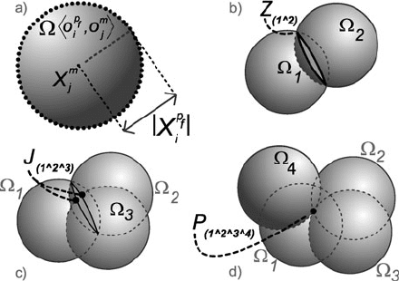
Fig. 6 (a) Constrained-sub-

space embodies the surface of

the sphere. (b) Cooccurring

constrained-subspaces

depicting a circle. (c)Three

constrained-subspaces acting

in conjunction yielding to a

point pair. (d) Four

constrained-subspaces

yielding to a simultaneity

point, i.e., the point within the

intersection of these four

constrained-subspaces

centered at X

with radius X

, see Fig. 6(a).

Note that the sphere in (4) is an element of the conformal geometric space PK

which has the Clifford algebra signature G

(4,1)

,see[5].

For a single percept, this idea provides no beneﬁt, but on second thought, when

observing the same concept with two different percepts, it turns out to be a very

proﬁtable formulation because the ego-center should reside in both constrained sub-

spaces, meaning that it has to be on the surface of both spheres at the same time.

Consider two restriction spheres simultaneously constraining the position of the

robot,





and Ω





;

they implicate that the position of the robot belongs to both subspaces. Thus, the

restricted subspace is a circle, i.e., an intersection of spheres, see Fig. 6(b),

(1∧2)

=Ω





∧Ω





Following the same pattern, a third sphere Ω

enforces the restriction to a point

pair

(1∧2∧3)

(1∧2)

∧Ω





i.e., circle–sphere intersection, see Fig. 6(c). Finally, a fourth sphere Ω

determines

the position of the robot, i.e., the intersection point from the latter point pair, see

Fig. 6(d),

(1∧2∧3∧4)

(1∧2∧3)

∧Ω





Latter concepts outline a technique which uses the previously partially matched

elements of the world model and process them by a geometric apparatus for generat-

ing the ego-center candidates. This apparatus uses the centers of the spheres within

the model space and the radii from the fused-percepts, see Fig. 2(6–9). The formu-

lation and treatment of the uncertainty acquired during perception is presented in

Sect. 3.

Model-Based Visual Self-localization Using Gaussian Spheres 309

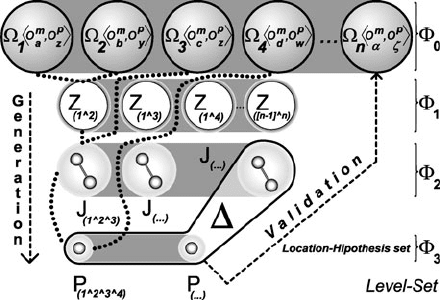
Fig. 7 Location hypotheses

generation–validation

mechanism systematically

manages the location

hypotheses

The computational complexity of this location hypotheses management process

is upper bounded by O(n

), where n is the cardinality of the subset of percept-

spheres. The amount of spheres n is never greater than 6 while generating candi-

dates; besides, in rare cases the internal partial result is that the intersection stages

are densely populated. This could be easily seen when intersecting two spheres. The

resulting circle occupies a smaller subspace which in successive stages meets only

fewer remaining spheres. One important factor why there are less operations in this

combinational computation is because the child primitives that result from the in-

tersection of parent spheres should not be combined with their relatives avoiding

useless computation effort and memory usage.

Hypotheses Generation

Each percept subgraph is used to produce the zero-level set, composed of spheres,

see Fig. 7,







ζ =1...n

These spheres are then intersected by means of the wedge operator ∧ in an upper

triangular fashion producing the ﬁrst-level set Φ

containing circles.

The second-level set Φ

is computed by intersecting the circles with spheres

from Φ

excluding those directly above. Then the latter resulting point-pairs are

intersected in the same way creating the highest possible level (third-level set) Φ

;

here the points resulting of the intersection of four spheres are contained.

Finally, elements of Φ

that have no descendants in Φ

and all elements on Φ

represent the location hypotheses

Δ :=







310 D. Gonzalez-Aguirre et al.

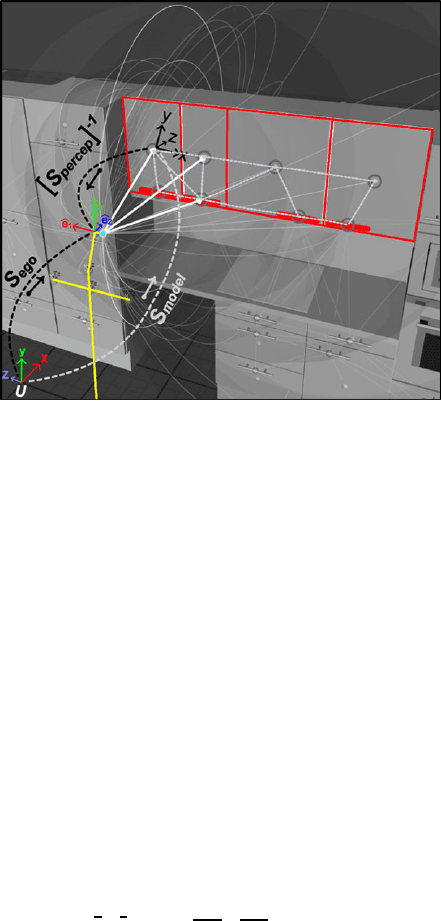
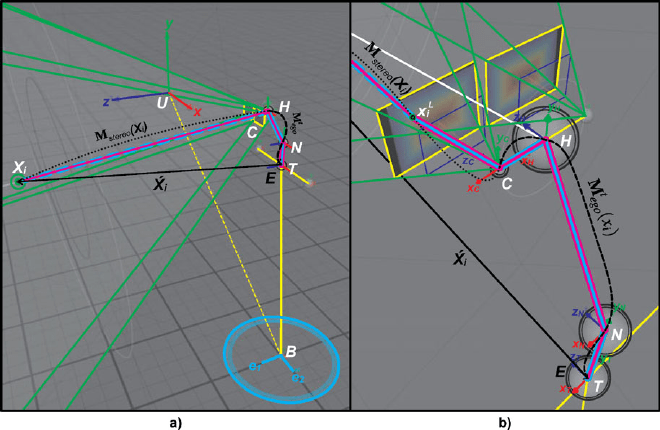
Fig. 8 Kinematic frames

involved in the ideal visual

self-localization. Notice the

directions of the coupling

transformations in order to

reveal the frame S

ego

Hypotheses Validation

Hypotheses are checked by selecting associations, see Figs. 2–8,





that were not considered in the generation of the current validating hypothesis. In

case there is more than one prevailing hypothesis, which rarely happens in nonsym-

metric repetitive environments, an active validation needs to take place selecting

objects from the model and then localizing them in the visual space. The criterion

to select the discriminator percept D

i,j

(priming instance) is the maximal pose dif-

ference between hypotheses pairs.

Ideal Pose Estimation

Once the location hypothesis has revealed, the position of the robot X

ego

(see Fig. 8)

and the orientation S

ego

are expressed as

ego



Self-Localization

= S

u,w,v

model



Model-Matching



i,j,k

Percept



−1

  

Visual-Perception

, (5)

which is actually the transformation from the kinematic chain that couples the

world-model frame S

model

(forwards) and the perception frame [S

i,j,k

Percept

]

−1

(back-

wards), see Fig. 8.

There are situations where a variety of diminishing effects alter the depth calcu-

lations of the percepts in a way that the ideal pose calculation may not be robust

Model-Based Visual Self-localization Using Gaussian Spheres 311

or could not be assessed. The subsequent sections describe the sources and nature

of the uncertainties, which are modeled and optimized by the proposed technique

to determine the optimal location of the robot, i.e., the maximal probabilistic posi-

tion.

3 Uncertainty

The critical role of the uncertainty cannot only strongly diminish the precision of

the estimated pose, but it can also prevent the existence of it by drawing away the

intersection of the restriction subspaces, i.e., the spheres might not intersect due to

numerical instability and errors introduced by the perception layer.

In order to sagaciously manage these conditions and other derived side effects,

it is crucial to reﬂect upon the nature of the acquired uncertainties regarding this

localization approach. There are two remarkable categorical sources of uncertainty,

image-to-space and space-to-ego uncertainties.

3.1 Image-to-Space Uncertainty

Image-to-space uncertainty is obtained from the appearance-based vision recogni-

tion process. It begins with the pixel precision limitations, e.g., noise, discretization,

quantization, etc., and ends with the error limitations of the camera model and its

calibration, e.g., radial–tangential distortion and intrinsic parameters [16]. This un-

certainty could be modeled, according to the central limit theorem [17], as a normal

distribution where the standard deviation σ

is strongly related to the perception

depth ρ

∼

, (6)

where ζ>1 ∈ R is an empirical scalar factor depending on the resolution of the

images and the vergence angle of the stereo rig, whereas the perception depth

=(x

−C

) ·ˆe

(7)

depicts the distance between camera center C

and point in space x

along the stereo

rig normal vector ˆe

, see Fig. 9. This deviation model arises from the following

superposed facts: ﬁrst, considering only the monocular inﬂuence in each camera of

the stereo rig.

The surface patch A

on the plane perpendicular to the optical axis of the camera

imaged into a single pixel P

grows as function of the distance ρ

=ρ

tan





tan





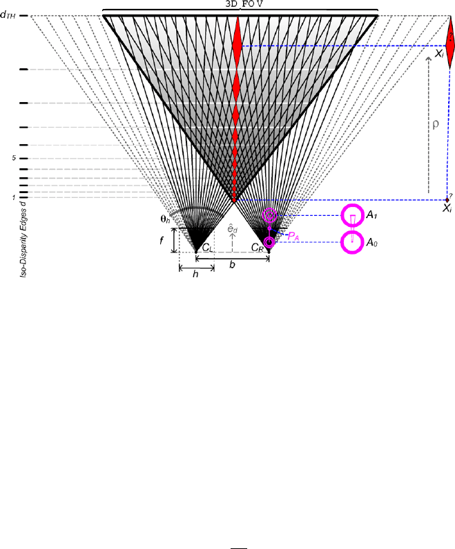
312 D. Gonzalez-Aguirre et al.

Fig. 9 The image-to-space uncertainty factors in a front-parallel conﬁguration

where θ

and θ

are the horizontal and vertical angular apertures of the ﬁeld of view,

whereas h and v depict the width and height resolutions of the image, see Fig. 9.

Consequently, the stereo triangulation has an additional effect during the estima-

tion of the 3D position M

stereo

) of a matched point pair. The distance ρ

affects

the magnitude of the disparity d

. Therefore, the precision of the pixel computations

plays a decisive role, i.e., the 3D space points which are closer to the base line have

wider disparities along the epipolar lines, meanwhile the points located after dis-

tance ρ

>fbhave a very narrow disparity, falling in the subpixel domain d<1,

which results in inaccurate depth calculations.

This situation also produces a sparse distribution of the iso-disparity surfaces

[15], meaning that the subspace contained between this surface-strata grows as

, (8)

where the focal distance f and the base line size b play relevant roles in the mea-

surement precision

b =C

−C

.

Figure 9 shows the ideal front parallel case iso-disparity edges delineating the

subspaces contained between two discrete steps in the disparity relation of (8).

In this manner, points contained within one of these subspaces produce the same

discrete disparity when matching corresponding pixels. Hence, the location uncer-

tainty should be proportional to the distance contained between iso-disparity sur-

faces. These two applied factors produce an uncertainty growing in an attenuated

Model-Based Visual Self-localization Using Gaussian Spheres 313

Fig. 10 The space-to-ego uncertainty acquisition process produced by the mapping of percepts

from camera coordinates to the ego-frame. (a) The whole transformation

ego

stereo

)).

(b) The transformation M

ego

=[T

(t)

]

−1

quadratic fashion, which is reﬂected in the model as a deviation spreading in the

same pattern reﬂected upon (7).

3.2 Space-to-Ego Uncertainty

The space-to-ego uncertainty is caused while relating the pose of the percepts from

the left camera frame to the ego-frame, i.e., head-base frame of the humanoid robot,

see Fig. 10(a).

It is caused by the physical and measurement inaccuracies, which are substan-

tially magniﬁed by projective effects, i.e., the almost negligible errors in the en-

coders and mechanical joints of the active head of the humanoid robot are ampliﬁed

proportionally to the distance ρ

between the ego-center and the location of the per-

cept.

Figure 10(b) shows the kinematic chain starting at x

, the left camera coordinates

of the space point X

. Subsequently, the transformation from the left camera frame

to the shoulders base T(t)passing through the eyes base H and neck frame N(t)

is given by

= M

ego

), (9)

ego

=[T

(t)

]

−1

, (10)

314 D. Gonzalez-Aguirre et al.

where M

ego

is the ego-mapping at time t. Here, the transformations T

(t)

and N

(t)

are time-dependent because they are active during the execution of the scanning

strategy, see Fig. 10(b).

4 Geometry and Uncertainty Model

Once the visual recognition components have provided all classiﬁed percepts within

a discrete step of the scanning trajectory, these percepts are mapped into the refer-

ence ego-frame using (9). This ego-frame is ﬁxed during the scanning phase. In this

fashion all percepts from different trials are located in a static common frame, see

Fig. 10(b).

The uniﬁcation-blending process done by the fusion phase simultaneously allows

the rejection of the percepts that are far from being properly clustered and creates

the delineation set which is later melted into a fused percept.

Next, the geometric and statistical phase for determining the position of the robot

based on intersection of spheres is properly formulated by introducing the Gaussian

sphere and its apparatus for intersection-optimization.

4.1 Gaussian Spheres

The considered restriction spheres Ω

are endowed with a soft density function



f(Ω

,x), Ω

∈PK

,x∈R

→(0, 1]∈R.

The density value decreases exponentially as a function of the distance from an

arbitrary point x to the surface of the sphere Ω

S(x,X

) =





x −X

−r





, (11)



f(Ω

,x)= e

−S(x,X

)

2σ

. (12)

The latter function depicts the nonnormalized

radial normal distribution



μ :=



x |ker



S(x,X

)



,σ



for x to be in the surface of Ω

, i.e., the null space of S(x,X

). Note that here the

standard deviation σ

refers to (6).

The density of a point x in relation with a sphere Ω

represents the nonnormal-

ized probability for the point x to belong to the surface of the sphere Ω

. Obviously

the maximal density is on the surface of the sphere itself.

By the factor

√

2π

Model-Based Visual Self-localization Using Gaussian Spheres 315

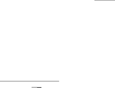
Fig. 11 Gaussian spheres meeting. (a) Two Gaussian spheres meeting Ω

∧ Ω

describing a

density-subspace Δ(Ω

∧Ω

).(b) Three Gaussian spheres Ω

i=1,2,3

meeting in two regions de-

picting a subspace Ω

∧ Ω

.(c) Detailed view of one of the previous subspaces. (d)Dis-

crete approximation of the maximal density location x

.(e) Details of the implicit density-space

Δ(Ω

∧Ω

).(f)(Upper-right) Implicit radius r

when estimating the density at position x

It is necessary to propose an effective mechanism which applies intersections

of restriction spherical subspaces as the essential idea for determining the robot

position. The nature of the applied intersection has to consider the endowed spatial

density of the involved Gaussian spheres.

In the following sections, the restriction spheres and their conjuncted composi-

tion properly model both uncertainties, allowing the meeting of spheres by ﬁnding

the subspace where the maximal density is located, see Fig. 11.

This could be interpreted as an isotropic dilatation or contraction of each sphere

in order to meet at maximal density of the total density function, see Figs. 12

and 13.

316 D. Gonzalez-Aguirre et al.

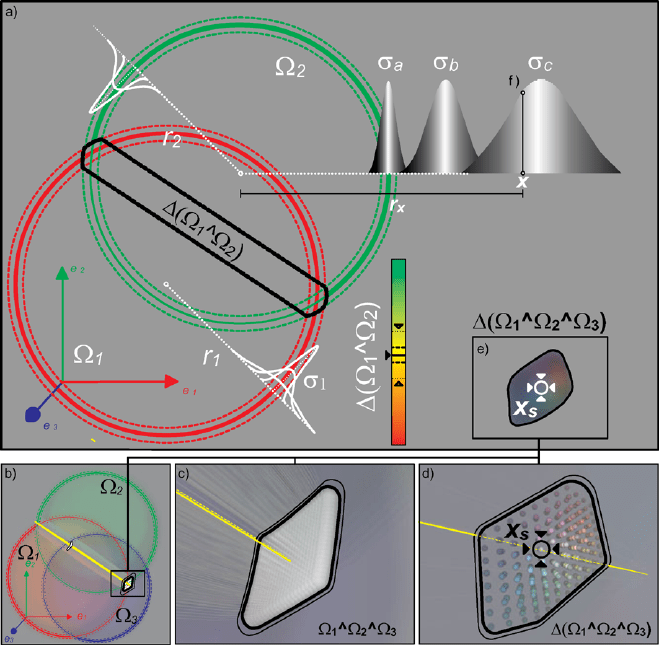
Fig. 12 Gaussian circles, i.e., 2D Gaussian spheres. (a) Three Gaussian circles setup. (b)Thetotal

accumulative density



(x) =





f(Ω

,x) allows a better visualization of the composition of its

product counterpart



(x), see also Fig. 13.(c) Density contours with seeds and their convergence

by means of gradient ascendant methods

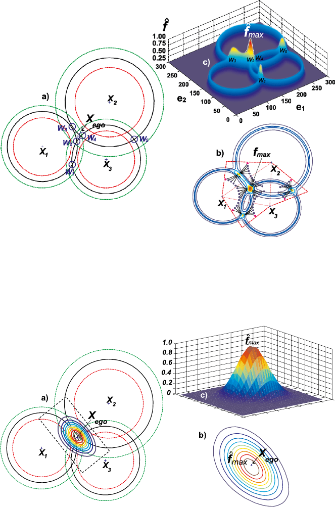
Fig. 13 The Gaussian circles, i.e., 2D Gaussian spheres. (a) Three Gaussian circles setup. (b)The

total density



(x) =





f(Ω

,x).(c) Density contours and ego-center X

ego

; notice that the re-

sulting distribution is not Gaussian

Model-Based Visual Self-localization Using Gaussian Spheres 317



(x) −→ (0, 1]∈R,x∈ R

, (13)



(x) =





f(Ω

,x). (14)

Due to the geometric structure composed by n spheres, it is possible to foresee

the amount of peaks and the regions W

where the density peaks are located, see

Fig. 12(c). Therefore, it is feasible to use state-of-the-art gradient ascendant methods

[18] to converge to the modes using multiple seeds. These should be strategically

located based on the spheres centers and intersection zones, see Fig. 12(b).

Finally, the seed with maximal density represents the solution position x

=argmax



(x). (15)

However, there are many issues of this shortcoming solution. The iterative solu-

tion has a precision limited by the parameter used to stop the shifting of the seeds. In

addition, the location and spreading of the seeds could have a tendency to produce

undesired oscillation phenomena, under- or oversampling and all other disadvan-

tages that iterative methods present.

The optimization expressed by (15) could be properly solved in a convenient

closed form. In order to address the solution x

, it is necessary to observe the con-

ﬁguration within a more propitious space, which simultaneously allows an advanta-

geous representation of the geometrical constraint and empowers an efﬁcient treat-

ment of the density, i.e., incorporating the measurements according to their uncer-

tainty and relevance while avoiding density decay.

4.2 Radial Space

The key to attain a suitable representation of the latter optimization resides in the

exponent of (12). There, the directed distance from a point x to the closest point on

the surface of the sphere is expressed by (11). When considering the total density

function, see (14), it unfolds the complexity by expressing the total density as a

tensor product.

The inherent nature of the problem lies in the radial domain, i.e., the expression

S(x,X

)

is actually the square magnitude of the difference between the radius r

and the implicit deﬁned radius r

between the center of the spheres X

and the point

x, see Fig. 11(f). Hence, the optimization conﬁguration can be better expressed in

radial terms, and the geometrical constraints restricting the relative positions of the

spheres are properly and naturally clariﬁed in the following sections.

4.3 Restriction Lines

Consider the case of two spheres Ω

and Ω

, see Fig. 14(a). Here, the radii of both

spheres and the distance between their centers