Bhadeshia H.K.D.H. Bainite In Steels. Transformations, Microstructure and Properties
Подождите немного. Документ загружается.

It follows that the nucleation rate must increase as the austenite grain size
decreases. If this is the only effect then the overall rate of transformation
must increase as
L decreases.
There is, however, another effect since the maximum volume V
S
max
of a sheaf
which starts from each grain boundary nucleus must be constrained by the
grain size, i.e.
V
S
max
/ L
3
If this effect is dominant then the overall rate will decrease as the austenite
grain size is reduced. Thus, it has been demonstrated experimentally that there
is an acceleration of transformation rate as
L is reduced when the overall
Kinetics
167
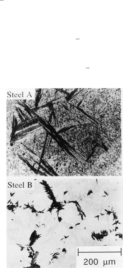
Fig. 6.28 (a) Bainite in a steel where nucleation is sparse and sheaf-growth is rapid.
The austenite grains constrain the amount of transformation that each nucleus can
cause. Reducing the austenite grain size then causes a net reduction in the overall
rate of transformation. (b) Bainite in a steel where the growth rate is small so that
the effect of the austenite grain size is simply to promote the nucleation rate. After
Matsuzaki and Bhadeshia (1999).
reaction is limited by a slow growth rate, i.e. when the sheaf volume remains
smaller than V
S
max
and hence is unconstrained by the grain size. Conversely, for
rapid growth from a limited number of nucleation sites, a reduction in the
austenite grain size reduces the total volume transformed per nucleus and
hence retards the overall reaction rate. The two circumstances are illustrated
in Fig. 6.28.
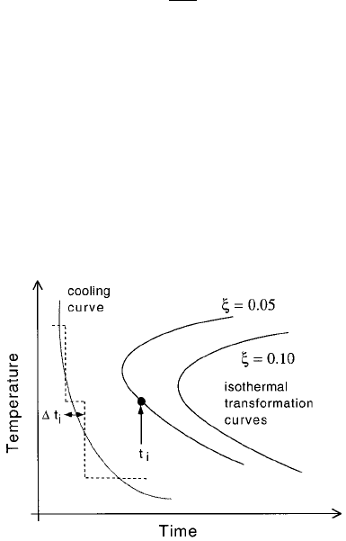
6.10.4 Anisothermal Transformation Kinetics
A popular method of converting between isothermal and anisothermal trans-
formation data is the additive reaction rule of Scheil (1935). A cooling curve is
treated as a combination of a suf®ciently large number of isothermal reaction
steps. Referring to Fig. 6.29, a fraction 0:05 of transformation is achieved
during continuous cooling when
X
i
t
i
t
i
1 6:49
with the summation beginning as soon as the parent phase cools below the
equilibrium temperature.
The rule can be justi®ed if the reaction rate depends solely on and T.
Although this is unlikely, there are many examples where the rule has been
empirically applied to bainite with success (e.g. Umemoto et al:, 1982).
Reactions for which the additivity rule is justi®ed are called isokinetic, imply-
ing that the fraction transformed at any temperature depends only on time and
a single function of temperature (Avrami, 1939; Cahn, 1956).
Bainite in Steels
168
Fig. 6.29 The Scheil method for converting between isothermal and anisothermal
transformation data.

6.11 Simultaneous Transformations
A simple modi®cation for two precipitates ( and ) is that equation 6.43
becomes a coupled set of two equations,
dV
1
V
V
V
dV
e
and dV
1
V
V
V
dV
e
6:50
This can be done for any number of reactions happening together (Robson and
Bhadeshia, 1997; Jones and Bhadeshia, 1997). The resulting set of equations
must in general be solved numerically, although a few analytical solutions are
possible for special cases which we shall now illustrate (Kasuya et al:, 1999).
6.11.1 Special Cases
For the simultaneous formation of two phases whose extended volumes are
related linearly:
V
e
BV
e
C with B 0andC 0 6:51
then with
i
V
i
=V, it can be shown that
exp
1 BV
e
C
V
dV
e
V
and
B
6:52
If the isotropic growth rate of phase is G and if all particles of start
growth at time t 0 from a ®xed number of sites N
V
per unit volume then
V
e
N
V
4
3
G
3
t
3
. On substitution of the extended volume in equation 6.52
gives
1
1 B
exp
C
V
1 exp
1 BN
V
4
3
G
3
t
3
V
with
B
6:53
The term expfC=Vg is the fraction of parent phase available for transforma-
tion at t 0; it arises because 1 expfC=Vg of exists prior to commence-
ment of the simultaneous reaction at t 0. Thus,
is the additional fraction of
that forms during simultaneous reaction. It is emphasised that C 0. A case
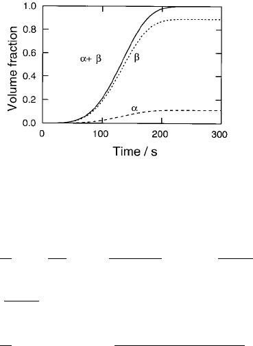
for which C 0andB 8 is illustrated in Fig. 6.30.
For the case where the extended volumes are related parabolically (Kasuya
et al:, 1999):
Kinetics
169
exp
C
V
4A
r
exp
1 B
2
4A
erf
1 B
4A
p
A
p
V
e
erf
1 B
4A
p
exp
C
V
1 exp
AV
e
2
1 BV
e
V
6:54
The volume fractions
i
again refer to the phases that form simultaneously and
hence there is a scaling factor expfC=Vg which is the fraction of parent phase
available for coupled transformation to and .
6.11.2 Precipitation in Secondary Hardening Steels
Whereas the analytical cases described above are revealing, it is unlikely in
practice for the phases to be related in the way described. This is illustrated for
secondary hardening bainitic and martensitic steels of the kind used com-
monly in the construction of power plant. The phases interfere with each
other not only by reducing the volume available for transformation, but also
by removing solute from the matrix and thereby changing its composition. This
change in matrix composition affects the growth and nucleation rates of all the
participating phases.
The calculations must allow for the simultaneous precipitation of M
2
X,
M
23
C
6
,M
7
C
3
,M
6
C and Laves phase. M
3
C is assumed to nucleate instanta-
neously with the paraequilibrium composition. Subsequent enrichment of
M
3
C as it approaches its equilibrium composition is accounted for. All the
phases, except M
3
C, are assumed to form with compositions close to equili-
Bainite in Steels
170
Fig. 6.30 Simultaneous transformation to phases 1 and 2 with C 0 and
B 8.
brium. The driving forces and compositions of the precipitating phases are
calculated using standard thermodynamic methods.
The interaction between the precipitating phases is accounted for by con-
sidering the change in the average solute level in the matrix as each phase
forms. This is frequently called the mean ®eld approximation. It is necessary
because the locations of precipitates are not predetermined in the calculations.
A plot showing the predicted variation of volume fraction of each precipitate
as a function of time at 600 8C is shown in Fig. 4.16. It is worth emphasising that
there is no prior knowledge of the actual sequence of precipitation, since all
phases are assumed to form at the same time, albeit with different precipitation
kinetics. The ®tting parameters common to all the steels are the site densities
and interfacial energy terms for each phase. The illustrated dissolution of
metastable precipitates is a natural consequence of changes in the matrix che-
mical composition as the equilibrium state is approached.
Consistent with experiments, the precipitation kinetics of M
23
C
6
are pre-
dicted to be much slower in the 2.25Cr1Mo steel compared to the 10CrMoV
and 3Cr1.5Mo alloys. One contributing factor is that in the 2.25Cr1Mo steel a
relatively large volume fraction of M
2
XandM
7
C
3
form prior to M
23
C
6
. These
deplete the matrix and therefore suppress M
23
C
6
precipitation. The volume
fraction of M
2
X which forms in the 10CrMoV steel is relatively small, so
there remains a considerable excess of solute in the matrix, allowing M
23
C
6
to precipitate rapidly. Similarly, in the 3Cr1.5Mo steel the volume fractions of
M
2
XandM
7
C
3
are insuf®cient to suppress M
23
C
6
precipitation to the same
extent as in the 2.25Cr1Mo steel.
It is even possible in this scheme to treat precipitates nucleated at grain
boundaries separately from those nucleated at dislocations, by taking them
to be different phases in the sense that the activation energies for nucleation
will be different.
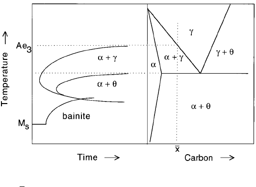
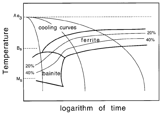
6.11.3 Time-Temperature-Transformation (TTT) Diagrams
Transformation curves on TTT diagrams tend to have a C shape because reac-
tion rates are slow both at high and at low temperatures. The diffusion of
atoms becomes dif®cult at low temperatures whereas the driving force for
transformation is reduced as the temperature is raised. The phase diagram
thus sets the thermodynamic limits to the decomposition of austenite (Fig. 6.31).
Most TTT diagrams can be considered to consist essentially of two C curves,
one for high temperatures representing reconstructive transformations to fer-
rite or pearlite. The other is for the lower temperatures where substitutional
atoms take too long to diffuse, so that reconstructive transformations are
replaced by displacive transformations such as Widmansta
È
tten ferrite and
Kinetics
171
bainite. The martensite-start temperature generally features on a TTT diagram
as a horizontal line parallel to the time axis (Cohen, 1940).
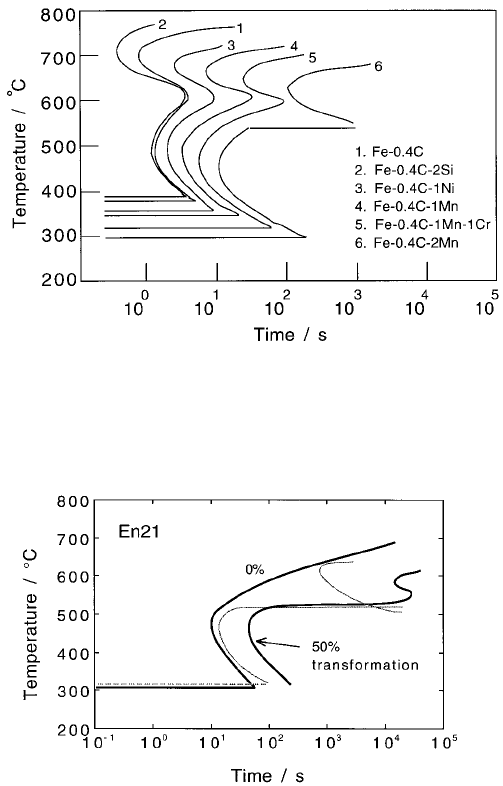
There are two major effects of alloying additions on transformation kinetics.
Solutes which decrease the driving force for the decomposition of austenite
retard the rate of transformation and cause both of the C curves to be displaced
to longer times. At the same time they depress the martensite-start temperature
(Fig. 6.32). The retardation is always more pronounced for reconstructive reac-
tions where all atoms have to diffuse over distances comparable to the size of
the transformation product. This diffusional drag exaggerates the effect of
solutes on the upper C curve relative to the lower C curve.
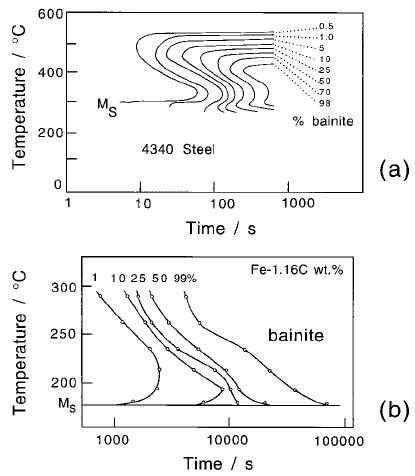
For steels where the reaction rate is rapid, it becomes dif®cult experimentally
to distinguish the two C curves as separate entities. For plain carbon and very
low-alloy steels, the measured diagrams take the form of just a single C curve
over the entire transformation temperature range. This is because the different
reactions overlap so much that they cannot easily be distinguished using con-
ventional experimental techniques (Hume-Rothery, 1966). Careful experiments
have shown this interpretation to be correct (Brown and Mack, 1973; Kennon
and Kaye, 1982). Sometimes the degree of overlap between the different trans-
formation products decreases as the volume fraction of transformation
increases (Fig. 6.33). This is because the partitioning of solute into austenite
has a larger effect on reconstructive transformations.
As predicted by Zener (1946), when the two curves can be distinguished
clearly, the lower C curve has a ¯at top. This can be identi®ed with the
Widmansta
È
tten ferrite-start or bainite-start temperature, whichever is the lar-
ger in magnitude (Bhadeshia, 1981a).
Bainite in Steels
172
Fig. 6.31 The relationship between a TTT diagram for a hypoeutectoid steel with a
concentration
x of carbon, and the corresponding Fe-C phase diagram.
There is more detail than implied in the two C curve description. The upper
and lower bainite reactions can be separated on TTT diagrams (Schaaber, 1955;
White and Owen, 1961; Barford, 1966; Kennon, 1978; Bhadeshia and Edmonds,
1979a). There is even an acceleration of the rate of isothermal transformation
just above the classical M
S
temperature, due to the formation of isothermal
Kinetics
173
Fig. 6.32 Calculated TTT diagrams showing the C-curves for the initiation of
reactions for a variety of steels.
Fig. 6.33 TTT diagram for Steel En21 (BISRA, 1956). The continuous lines are
experimental. The separation of the two constituent C curves, which is not appar-
ent for the 0% curve is revealed as the extent of reaction increases. The dashed
curves are calculated for 0% transformation.
martensite (Howard and Cohen, 1948; Schaaber, 1955; Radcliffe and Rollason,
1959; Smith et al:, 1959; Brown and Mack, 1973a,b; Babu et al:, 1976; Oka and
Okamoto, 1986, 1988).
Isothermal martensite plates tend to be very thin and are readily distin-
guished from bainite. Although the overall rate of martensitic transformation
appears isothermal, the individual plates are known to grow extremely
rapidly. The isothermal appearance of the overall reaction is therefore due to
the nucleation process (Smith et al:, 1959). The stresses caused by bainitic
transformation seem to trigger induced isothermal martensite. The rate even-
tually decreases as the transformation temperature is reduced below the M
S
temperature, giving the appearance of a C-curve with the peak transformation
rate located below M
S
(Fig. 6.34).
6.11.4 Continuous Cooling Transformation (CCT) Diagrams
Steels are not usually isothermally transformed. It is more convenient to gen-
erate the required properties during continuous cooling from the austenitic
Bainite in Steels
174
Fig. 6.34 (a) TTT diagram for a Fe±0.39C±0.70Mn±1.7Ni±0.76Cr±0.2Mo±0.28Si±
0.22Cu wt% alloy austenitised at 900 8C for 15 minutes. Note the acceleration in
the rate of transformation as the M
S
temperature is approached (data from Babu
et al:, 1976). (b) Similar data for a plain carbon steel (Howard and Cohen, 1948).
condition. Continuous-cooling-transformation (CCT) diagrams are then used
to represent the evolution of microstructure (Fig. 6.35).
The rate of transformation in a given steel with a known austenite grain size
can be described with just one TTT diagram. However, a different CCT dia-
gram is required for cooling function, e.g. whether the cooling rate is constant
or Newtonian. It is therefore necessary to plot the actual cooling curves used in
the derivation of the CCT diagram (Fig. 6.35). Each cooling curve must begin at
the highest temperature where transformation becomes possible (usually the
Ae
3
temperature).
Each CCT diagram requires a speci®cation of the chemical composition of
the steel, the austenitisation conditions, the austenite grain size and the cooling
condition. The diagrams are therefore speci®c to particular processes and lack
the generality of TTT diagrams.
The CCT diagram is usually partitioned into domains of microstructure; Fig.
6.35 shows the conditions under which bainite and ferrite form. Mixed micro-
structures are obtained when a domain boundary is intersected by a cooling
curve. The constant volume fraction contours must be continuous across the
domain boundaries to avoid (incorrect) sudden changes in volume fraction as
the boundary is crossed (e.g. points a, b on Fig. 6.36). The contours represent
the fraction of austenite which has transformed into one or more phases. It
follows that there are constraints on how the zero percent martensite and
bainite curves meet, avoiding the double intersection with the cooling curve
illustrated in Fig. 6.36b,c. Cooling curve X which leads to a fully martensitic
Kinetics
175
Fig. 35 CCT diagram illustrating the cooling curves, constant volume percent
contours and transformation temperatures.
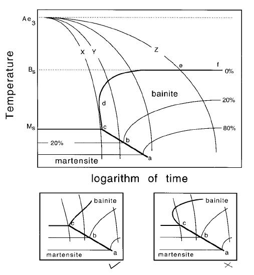
microstructure, intersects the 0% transformation curve at just one point, with-
out intersecting the region cd. Cooling curve Y, on the other hand, produces a
mixed microstructure with less than 20% of bainite, the remaining austenite
transforming to martensite on cooling. The temperature at which martensitic
transformation begins (line abc) is depressed if bainite forms ®rst and enriches
the residual austenite with carbon.
The bainite curve in Fig. 6.36 approaches the B
S
temperature asymptotically
along ef as the cooling rate decreases consistent with the ¯at top of the bainite
C curve in the TTT diagram. This is not always the case as shown schematically
in Fig. 6.37. (Kunitake, 1971; Schanck, 1969; Lundin et al:, 1982). Any transfor-
mation which precedes bainite alters the chemical composition of the residual
austenite. The main changes occur in the region associated with the vertical
line `c' in Fig. 6.37 The temperature at which the bainite ®rst forms is depressed
by the changed composition of the austenite. Because the ferrite and bainite
domains are separated by a time gap, the continuity of constant volume
fraction contours is interrupted. The contours must still be plotted so that
Bainite in Steels
176
Fig. 6.36 Schematic CCT diagrams illustrating the continuity of constant volume
percent contours across microstructure domain boundaries and the correct way in
which the zero percent curves of different domains must meet at the point c.