Bhattacharjee J.K., Bhattacharyya S. Non-Linear Dynamics Near and Far from Equilibrium
Подождите немного. Документ загружается.


1 Introduction 19
Weround offour discussion of response functions by looking at the entropy which is
the response to atemperature fluctuation. The entropy is defined as S =−
∂F
∂T
)
V
with
the external field equal to zero. With m
2
=a
0
(T −T
c
), we can write S =−a
0
∂F
∂m
2
=
a
0
φ
2
(r)d
D
r. A further derivative yields the specific heat as C =T
∂S
∂T
=T
∂S
∂m
2
.
This leads to
C = a
2
0
T
1
Z
d
D
r
1
d
D
r
2
φ
2
(r
1
)φ
2
(r
2
)e
−
d
D
r [
m
2
2
φ
2
+
1
2
(
∇φ)
2
+
λ
4
φ
4
]/k
B
T
c
−
1
Z
2
d
D
r
1
φ
2
(r
1
)e
−
d
D
r [
m
2
2
φ
2
+
1
2
(
∇φ)
2
+
λ
4
φ
4
]/k
B
T
c
2
= a
2
0
T
φ
2
(r
1
)φ
2
(r
2
)
c
d
D
r
1
d
D
r
2
a
2
0
T
c
φ
2
(r
1
)φ
2
(r
2
)
c
d
D
r
1
d
D
r
2
(1.0.62)
where the subscript c denotes the connected part. To get a feel for how Eq.(1.0.62)
works, we can approximate the connected correlation (i.e. r
1
and r
2
are connected)
as
φ
2
(r
1
)φ
2
(r
2
)
c
φ(r
1
)φ(r
2
)
2
,
and use the asymptotic form of
φ(r
1
)φ(r
2
)
e
−r
12
/ξ
r
D−2
12
to obtain
C ∝V
d
D
r
12
e
−2 r
12
/ξ
r
2D−4
12
∝ξ
4−D
∝(T −T
c
)
4−D
2
(1.0.63)
Here is another response function which diverges as the correlation length becomes
infinitely big. The relevant exponent (generally denoted by α)
C =C
0
|T −T
c
|
−α
(1.0.64)
is in the approximation α =
4−D
2
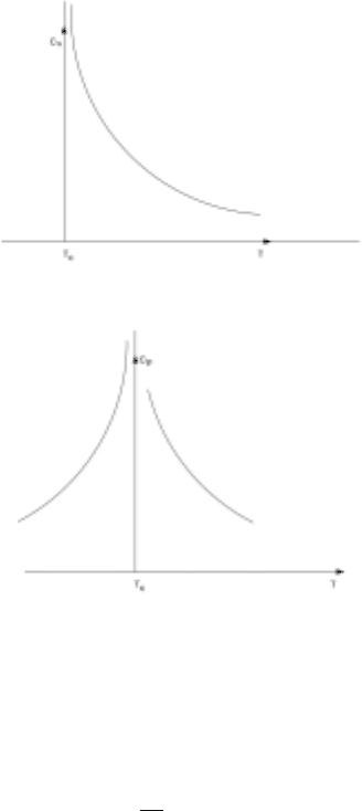
. The divergent specific heat at the liquid-gas
critical point is shown in Fig. 1.9a. It also diverges near the superfluid transition
in liquid He
4
Fig. 1.9b. The exponents however are different from
4−D
2
, for the
liquid-gas system α 0.11 while for the superfluid transition α 0.
20 1 Introduction
Figure 1.9. Constant volume specific heat near the liquid gas critical point.
Figure 1.9. Constant pressure specific heat near the superfluid transition.
We can also find the specific heat from the approximation of Eq.(1.0.37). In
this case
F = 0 for T>T
c
and F =−
a
2
0
2λ
for T<T
c
(1.0.65)
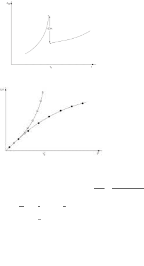
This implies a discontinuity in the measured specific heat which will be a combi-
nation of the critical and non-critical parts (see Fig. 1.10).
If we compare this with the specific heat near the superconducting transition,
Fig. 1.11, then the similarity is striking. We now have a situation which may
appear contradictory. The liquid-gas transition, the superfluid transition and the
superconducting transition are all second order transitions. In the way we handled
the Landau-Ginzburg free energy, the specific heat diverged at the critical point
while in the mean-field approximation, the specific heat has a discontinuity at
T =T
c
. The specific heat at the liquid-gas and superfluid transitions diverge at
the critical point but remains finite with a discontinuity at the superconducting
transition. To understand the differing behaviours, we need to understand the role
of fluctuations. In the mean field approach, where the fluctuating field φ(r) is
1 Introduction 21
Figure 1.10. Jump in the mean field specific heat
Figure 1.11. Experimental specific heat near the supercondfucting transition
replaced by the spatially uniform m, the role of fluctuations is minimal. The role of
fluctuations is characterized by the correlation length ξ =
1
|a|
1/2
=
1
a
1/2
0
|T −T −c|
1/2
.
There is another length scale in the problem which is characterized by the coupling
constant λ. Since
d
D
r [
m
2
2
φ
2
+
1
2
(
∇φ)
2
+
λ
4
φ
4
] appears in the exponent of an
exponential, every term in it must be dimensionless (in units where K
B
T =1) we
find that φ has the dimension L
1−
D
2
where L is a length (from the middle term).
The last term now shows that λ has the dimension L
D−4
giving a length scale λ
1
D−4
.
At a particular temperature T
m
the correlation length becomes the same as the
other length scale and for smaller values of T −T
c
, the fluctuations break up the
order. The mean field theory is valid if
T −T
c
≥
1
a
0
λ
2
4−D
=
1
a
0
ξ
2
0
(1.0.66)
where ξ
0
is a non-critical characteristic length. If ξ
0
is very big, then the condition
of Eq.(1.0.67) is satisfied for almost all T and the system shows the mean field
exponents. This is true for the superconducting transition where the pair coherence
length ξ
0
is the non-critical length scale and is extremely big. This is the reason
22 1 Introduction
behind the excellent agreement between the theory and experiment in Figs.1.10
and 1.11. For other systems which have a much smaller value of ξ
0
, there will be a
temperature T
m
where the equality of Eq.(1.0.67) holds and if one is further away
from T
c
than T
m
, then the mean field exponents will be observed. Closer to T
c
than
T
m
, the exponents will change and the phenomenon is called crossover. Writing
Eq.(1.0.67) as
[a
0
(T −T
c
)]
4−D
≥λ
2
(1.0.67)
we see that for T T
c
, this relation will always be satisfied for D>4. Thus mean
field results are always true for D>4. It is for D<4, that the crossover occurs
from mean field to nontrivial exponents. If we are measuring the compressibility
of a fluid or susceptibility of a uniaxial magnet, then for temperatures very close
to T
c
, γ 1.24 is observed while further away one finds γ =1. Similarly, for the
magnetization it is β 0.32 very close to T
c
and β =0.5 somewhat further away.
For the exponent δ,itisδ 5 for very small magnetic fields and δ 3 for large
fields. This brings up the final question : How does one calculate the nontrivial
exponents β 0.32, γ 1.24 and δ 5? Two exponents α and η are identically
zero in the mean field theory while experiments very closely show that α 0.11
for the fluid and η 0.04. These two small exponents are consequently crucial to
the theory. In Chapter 3, we will describe the technique which allows us to arrive
at non-trivial values for the critical exponents. The success in setting up a realistic
theory for second order phase transitions is the inspiration behind bringing together
various topics in dynamics of such macroscopic systems - both near equilibrium
and out-of-equilibrium - in the subsequent chapter.
References
1. H.E. Stanley Introduction to Phase Transitions and Critical Phenomena. Oxford
University Press, Oxford. (1971)
2. L.D. Landau and E.M.Lifshitz, Statistical Physics, Part 1(3rd Ed.). (Course of
Theoretical Physics, Vol.5). Pergamon Press, Oxford, (1980)
3. N. Goldenfeld,Lectures on Phase Transitionsand the Renormalization Group. Addison-
Wesley, Mass. (1992)
4. P. Pfeuty and G. Toulouse, Introduction to the Renormalization Group and Critical
Phenomena. Wiley, London. (1977)
5. J.M. Yeomans, Statistical Mechanics of Phase Transitions. Clarendon Press, Oxford.
(1992)
6. C. Domb and M.S. Green(eds.), Phase Transitions and Critical Phenomena, Vols. 5
and 6. Academic Press, New York. (1976)
7. J.J. Binney et.al., The Theory of Critical Phenomena, An Introduction to the Renor-
malization Group. Clarendon Press, Oxford. (1993)
8. D.J. Amit, Field Theory, the Renormalization Group and Critical Phenomena,
(2nd. Ed.) World Scientific, Singapore. (1984)
1 Introduction 23
9. P.M. Chaikin and T.C. Lubensky, Principles of Condensed Matter Physics. Cambridge
University Press. (1995)
10. J.L. Cardy, Scaling and renormalization in statistical physics. Cambridge University
Press. (1996)
11. G. Parisi, Statistical Field Theory. Addison-Wesley, New York. (1988)
12. S.K. Ma, Modern Theory of Critical Phenomena. Addison-Wesley. (1976)

2
Models of Dynamics
2.1 Introduction
Our concern will mainly be with mesoscopic systems. These are systems whose
length and time scales are significantly larger (a few orders of magnitude) than
atomic scales but still small compared to macroscopic scales (system size etc.). A
typical example is provided by a system near a second order phase transition point,
e.g. a magnet being cooled towards the Curie point. For temperatures far above the
Curie point the individual magnetic moments inside the magnet are moving around
randomly and the overall magnetization of the sample is zero. As the temperature
is lowered and the Curie point is approached, the individual magnetic moments
become more correlated. The energy is lowered if the moments are aligned and as
the temperature decreases, the entropy effects become smaller and the gradually
dominating energy part of the thermodynamic free energy causes the correlations
to build up. The distance over which the correlations exist is called the correlation
length ξ. As the temperature reaches the Curie point, the correlation length becomes
infinitely big, leading to correlation functions which become infinitely long ranged.
For temperatures very close to the critical point (say a millikelvin away from the
critical point), the correlation length is of the order of a few microns which is
about three or four orders of magnitude larger than the atomic scale which is of the
order of a few angstroms. This makes for an ideal mesoscopic system. If we are to
describe the statics or dynamics of such a system, the task would be quite difficult
if it were to be in terms of individual atoms or molecules. Consequently, one uses
a coarse grained description. One talks about the averaged magnetic moment at
any point of space. The averaging at any point of space is done over several atomic
dimensions and the result is a magnetization field m(r), in terms of which the
critical phenomena is described. The generic name for the field m(r) is the order
parameter field - φ(r). It could be the density fluctuation field for the liquid-vapour
26 2 Models of Dynamics
transition (or a binary fluid near its consolute point) or the superfluid fluctuations
(amplitude and phase) near the lambda point or the fluctuations in the staggered
magnetization near the antiferromagnetic transition.
Our interest, as we emphasized in the last chapter is in systems which are
described in terms of macroscopic fields. In this chapter, we will describe the
kind of dynamics that one expects for these systems. We begin with a system
near the critical point that we have discussed in the last chapter. If we are to
describe dynamics of this system, then the equation of motion is not so obvious.
Forone thing, those degreesof freedom which have been averagedover, are going to
influence the dynamics and this cannot be in a deterministic fashion. Consequently,
the dynamics will be described in terms of stochastic rather than deterministic
differential equations. The dynamics of the fluctuations is generally expected to be
relaxational as we expect a small fluctuation from the equilibrium state to disappear
in time. This relaxation generally is the linear part of the equation of motion -
the expectation is that the equation of motion will be first order in time since
specification of only the initial value of the order parameter should be enough to
specify its future dynamics. Thus the expected dynamics is of Langevin variety.
A different example is provided by crystal growth by ballistic deposition of
atoms. The depositing atoms diffuse across the surface to settle down at places
where the local energy is a minimum. This smooths out the growing surface. On
the other hand, there is intrinsic noise in the deposition process and this causes
the surface to be rough. The natural variable to describe the growth of this surface
is the local height variable h(r,t). Here r is the coordinate in the substrate. The
dynamics of the field h(r,t) has two clear cut parts:
• i) a surface diffusion which helps smooth out any fluctuation in h and
• ii) a noise part corresponding to the fluctuation in the deposition process
Thus, once more the dynamics is of the Langevin variety.
Yet another example of a mesoscopic system is the dynamics of polymer chains.
Consider a polymer chain put in a solvent. If the polymer is hydrophobic, then to
prevent contact with the water molecules the polymer tends to fold into a ball. The
entropyterm in the thermodynamic free energy would likethe polymer to spread out
and hence there is a competition between the energy and the entropy effects. As the
temperature is lowered, the chain is expected to undergo a transition into a compact
structure. The compact structure is typically of the order of microns (examples
of these compact structures are the enzyme like proteins) and constitute another
example of a mesoscopic system. The dynamics of a polymer chain is governed
again by a Langevin equation. For a randomly hydrophobic and hydrophillic chain,
thus the dynamics can be of some relevance to the interesting problem of protein
folding.
Finally, we mention the problem of turbulence. Here the randomness is gener-
ated by the non-linear term in the Navier-Stokes’ equation. However, to maintain
the turbulence we need to have a maintained mean flow and energy transfer has
to occur from the mean flow to the fluctuations. There would also be the question

2.2 Langevin Picture 27
of boundary conditions on the various bounding surfaces, however far away. It is
the information about boundaries and maintained mean flows that we can average
over and cast the Navier-Stokes’ equation as a Langevin equation with a fluctuating
force. We begin our discussion of Langevin equations by an explicit construction.
A single particle interacts with a set of particles which constitute a bath. It will be
demonstrated how averaging over the bath variables leads to the fluctuating force.
The derivation that follows is due to Zwanzig.
2.2 Langevin Picture
Without any loss of generality, we will confine ourselves to one dimensional dy-
namics. The bath will be a set of harmonic oscillators, each characterized by a
coordinate q
i
and a conjugate momentum p
i
. The particle whose equation of mo-
tion is our concern has a coordinate X, moves in a potential V(X) and interacts
with the bath via a quadratic coupling, i.e. a coupling of the form Xq
i
for all i. The
Hamiltonian describing the system is
H =
P
2
2
+V(X)+
i
1
2
ω
2
i
(q
i
−
γ
i
ω
2
i
X)
2
+
i
P
2
i
2
(2.2.1)
where all masses have been set to unity. Now the equation of motion for P is
˙
P =−
∂V
∂X
+
i
γ
i
(q
i
−
γ
i
ω
2
i
X) (2.2.2)
and that for q
i
is
¨q
i
+ω
2
i
q
i
=γ
i
X (2.2.3)
The solution for q
i
(t) can be written down as
q
i
(t) =q
i
(0)cosω
i
(t) +
p
i
(0)
ω
i
sinω
i
t +
t
0
γ
i
sinω
i
(t −s)
ω
i
X(s)ds
=q
i
(0)cosω
i
t +
p
i
(0)
ω
i
sinω
i
t +
γ
i
ω
2
i
X(t) −
γ
i
ω
2
i
X(0)cosω
i
t
−
t
0
γ
i
ω
2
i
cosω
i
(t −s)P(s)ds
leading to,
q
i
(t) −
γ
i
ω
2
i
X(t) =
q
i
(0) −
γ
i
ω
2
i
X(0)
cosω
i
t +
p
i
(0)
ω
i
sinω
i
t
−
t
0
γ
i
ω
2
i
cosω
i
(t −s)P(s)ds (2.2.4)
(note that
˙
X =P since m =1).

28 2 Models of Dynamics
Inserting this solution in Eq.(2.2.2), we have
˙
P =−
∂V
∂X
−
i
t
0
γ
2
i
ω
2
i
cosω
i
(t −s)P(s)ds
+
i
γ
i
(q
i
(0) −
γ
i
ω
2
i
X(0))cosω
i
t +
i
γ
i
ω
i
p
i
(0)sinω
i
t
=−
∂V
∂X
−
t
0
K(t −s)P(s)ds +f(t) (2.2.5)
where
K(t −s) =
γ
2
i
ω
2
i
cosω
i
(t −s)
and f(t) =
i
γ
i
q
i
(0) −
γ
i
ω
2
i
X(0)
cosω
i
t +
i
γ
i
ω
i
p
i
(0)sinω
i
t
(2.2.6)
As expected, at this point the equation of motion for P(t) is completely deter-
ministic. Note that the force f(t)is dependent on the initial values of all the bath
variables which would be of the order of the Avogadro number. Hence, practical
specification of the force is impossible. Consequently, it pays to go to a statistical
description. It is more convenient to think of f(t)as a stochastic force with only its
moments specified. To specify the moments, we require a distribution. In this case,
the distribution has to do with the distribution of the initial values of the coordi-
nates and momenta of the heat bath. If we assume that the system is characterized
by a temperature T , then the distribution is of Maxwell-Boltzmann variety (i.e.
Gaussian) and we have
P
q
i
−
γ
i
ω
2
i
X
, {p
i
}
=
ω
πK
B
T
N
N
i=1
exp
−
1
2
p
2
i
+
1
2
ω
2
i
q
i
−
γ
i
ω
2
i
X
2
/K
B
T
(2.2.7)
leading to the moments
p
i
(0)=q
i
(0) −
γ
i
ω
2
i
X(0)=0
p
i
(0)p
j
(0)=K
B
Tδ
ij
(q
i
(0) −
γ
i
ω
2
i
X(0))ω
2
i
(q
j
(0) −
γ
j
ω
2
j
X(0))=K
B
Tδ
ij
p
i
(0)(q
j
(0) −
γ
j
ω
2
j
X(0))=0 for all i and j (2.2.8)

2.2 Langevin Picture 29
We can now calculate the moments of the random force f(t). Clearly,
f(t)=0 (2.2.9)
As for the second moment
f(t)f(s)=
i
γ
i
q
i
(0) −
γ
i
ω
2
i
X(0)
cosω
i
t +
γ
i
ω
i
P
i
(0)sinω
i
t
×
γ
j
q
j
(0) −
γ
j
ω
2
j
X(0)
cosω
j
t +
γ
j
ω
j
P
j
(0)sinω
j
t
=
i,j
γ
i
γ
j
q
i
(0) −
γ
i
ω
2
i
X(0)
q
j
(0) −
γ
j
ω
2
j
X(0)
×
cosω
i
tcosω
j
s +
i,j
γ
i
γ
j
ω
i
ω
j
p
i
(0)p
j
(0)sinω
i
t sinω
j
s
=K
B
T
j
γ
2
j
ω
2
j
cosω
j
(t −s)
=K
B
TK(t−s) (2.2.10)
Let us return to Eq.(2.2.5) and examine the different forces on the R.H.S. The first
term, i.e.
∂V
∂X
, comes from an externally imposed potential while the second and
third terms come from the interaction with the environment. We will make the
assumption of being in the limit of large coupling between the particle and the bath
variables and drop the potential term
∂V
∂X
. The R.H.S of Eq.(2.2.5) now contains
two terms
• i) a damping term −
t
0
K(t −s)p(s)ds and
• ii) a random term f(t), such that f(t) and f(t)f(s)=K
B
TK(t−s)
An equation of this sort is called a Langevin equation - it has resulted entirely from
the interaction with the environment (we will see later that there can be additional
terms).
˙p =−
t
0
K(t −s)p(s)ds +f(t) (2.2.11)
In the particular example, we have chosen
f(t)f(s)=K
B
TK(t−s) (2.2.12)
relating the stochastic term to the dissipative term. This may not always happen.
We need to discuss the classification of noise. For a correlation of the kind
shown in Eq.(2.2.12), the noise at time t is correlated with the noise at time s. It
thus retains memory and is called a coloured noise. Returning to the expression