Birge J.R., Louveaux F. Introduction to Stochastic Programming

Подождите немного. Документ загружается.

24 1 Introduction and Examples

Solving the problem in (2.1) yields an optimal expected utility value of −1.514 . We

call this value, RP , for the expected recourse problem solution value. The optimal

solution (in thousands of dollars) appears in Table 6.

Table 6 Optimal solution with three-period stochastic program.

Period, Scenario Stock Bonds

1,1-8 41.5 13.5

2,1-4 65.1 2.17

2,5-8 36.7 22.4

3,1-2 83.8 0.00

3,3-4 0.00 71.4

3,5-6 0.00 71.4

3,7-8 64.0 0.00

Scenario Above G Below G

1 24.8 0.00

2 8.87 0.00

3 1.43 0.00

4 0.00 0.00

5 1.43 0.00

6 0.00 0.00

7 0.00 0.00

8 0.00 12.2

In this solution, the initial investment is heavily in stock ($41,500) with only

$13,500 in bonds. Notice the reaction to ﬁrst-period outcomes, however. In the case

of Scenarios 1 to 4, stocks are even more prominent, while Scenarios 5 to 8 reﬂect a

more conservative government security portfolio. In the last period, notice how the

investments are either completely in stocks or completely in bonds. This is a general

trait of one-period decisions. It occurs here because in Scenarios 1 and 2, there is no

risk of missing the target. In Scenarios 3 to 6, stock investments may cause one to

miss the target, so they are avoided. In Scenarios 7 and 8, the only hope of reaching

the target is through stocks.

We compare the results in Table 6 to a deterministic model in which all random

returns are replaced by their expectation.For that model, because the expected return

on stock is 1.155 in each period, while the expected return on bonds is only 1.13

in each period, the optimal investment plan places all funds in stocks in each period.

If we implement this policy each period, but instead observed the random returns,

we would have an expected utility called the expected value solution, or EV .Inthis

case, we would realize an expected utility of EV = −3.788 , while the stochastic

program value is again RP = −1.514 . The difference between these quantities is

the value of the stochastic solution:

VSS = RP−EV = −1.514 −(−3.788)=2.274 .

1.2 Financial Planning and Control 25

This comparison gives us a measure of the utility value in using a decision from a

stochastic program compared to a decision from a deterministic program. Another

comparison of models is in terms of the probability of reaching the goal. Models

with these types of objectives are called chance-constrained programs or programs

with probabilistic constraints (see Charnes and Cooper [1959] and Pr´ekopa [1973]).

Notice that the stochastic program solution reaches the goal 87.5% of the time. The

expected value deterministic model solution only reaches the goal 50% of the time.

In this case, the value of the stochastic solution may be even more signiﬁcant.

The formulation we gave in (2.1) can become quite cumbersome as the time

horizon, H , increases and the decision tree of Figure 3 grows quite bushy. Another

modeling approach to this type of multistage problem is to consider the full horizon

scenarios, s , directly, without specifying the history of the process. We then sub-

stitute a scenario set S for the random elements

. Probabilities, p(s) , returns,

(i,t,s) , and investments, x(i,t, s) , become functions of the H -period scenarios

and not just the history until period t .

The difﬁculty is that, when we have split up the scenarios, we may have lost

nonanticipativity of the decisions because they would now include knowledge of

the outcomes up to the end of the horizon. To enforce nonanticipativity, we add

constraints explicitly in the formulation. First, the scenarios that correspond to the

same set of past outcomes at each period form groups, S

,...,s

t−1

, for scenarios at

time t . Now, all actions up to time t must be the same within a group. We do this

through an explicit constraint. The new general formulation of (2.1) becomes:

maxz =

∑

p(s)(qy(s) −rw(s))

s. t.

∑

i=1

x(i,1,s)=b , ∀s ∈S , (2.2)

∑

i=1

(i,t,s)x(i,t −1,s) −

∑

i=1

x(i,t,s)=0 , ∀s ∈ S ,

t = 2,...,H ,

∑

i=1

(i,H,s)x(i,H,s) −y(s)+w(s)=G ,

⎛

⎝

∑



∈S

J(s,t)

p(s



)x(i,t,s



)

⎞

⎠

−

⎛

⎝

∑



∈S

J(s,t)

p(s



)

⎞

⎠

x(i,t,s)=0 ,

∀1 ≤ i ≤I , ∀1 ≤t ≤ H , ∀s ∈S ,

x(i,t,s) ≥ 0 , y(s) ≥ 0 , w(s) ≥ 0 ,

∀ 1 ≤ i ≤ I , ∀ 1 ≤t ≤ H , ∀ s ∈ S ,

where J(s,t)={s

,...,s

t−1

} such that s ∈ S

,...,s

t−1

. Note that the last equality

constraint indeed forces all decisions within the same group at time t to be the

same. Formulation (2.2) has a special advantage for the problem here because these

26 1 Introduction and Examples

nonanticipativity constraints are the only constraints linking the separate scenarios.

Without them, the problem would decompose into a separate problem for each s ,

maintaining the structure of that problem.

In modeling terms, this simple additional constraint makes it relatively easy to

move from a deterministic model to a stochastic model of the same problem. This

ease of conversion can be especially useful in modeling languages. For example,

Figure 4 gives a complete AMPL (Fourer, Gay, and Kernighan [1993]) model of

the problem in (2.2). In this language, set, param,andvar are keywords for sets,

parameters, and variables. The addition of the scenario indicators and nonanticipa-

tivity constraints (nonanticip) are the only additions to a deterministic model.

# This problem describes a simple ﬁnancial planning problem

# for ﬁnancing college education

set investments; # different investment options

param initwealth; # initial holdings

param H; # number of periods

param scenarios; # number of scenarios (total S)

# The following 0-1 array shows which scenarios are combined at period H

param scen

links { 1..scenarios,1..scenarios,1..H } ;

param target; # target value G at time H

param invest; # value of investing beyond target value

param penalty; # penalty for not meeting target

param return { investments,1..scenarios,1..H } ; # return on each inv

param prob { 1..scenarios } ; # probability of each scenario

# variables

var amtinvest { investments,1..scenarios,1..H } ¿= 0; #actual amounts inv’d

var above

target { 1..scenarios } ¿= 0; # amt above ﬁnal target

var below

target { 1..scenarios } ¿= 0; # amt below ﬁnal target

# objective

maximize exp

value : sum { i in 1..scenarios } prob[i]*(invest*above target[i]

- penalty*below

target[i]);

# constraints

subject to budget { i in 1..scenarios } :

sum { kininvestments} (amtinvest[k,i,1]) = initwealth;#invest initial wealth

subject to nonanticip { k in investments,j in 1..scenarios,t in 1..H } :

(sum { i in 1..scenarios } scen

links[j,i,t]*prob[i]*amtinvest[k,i,t]) -

(sum { i in 1..scenarios } scen

links[j,i,t]*prob[i])*

amtinvest[k,j,H] = 0; # makes all investments nonanticipative

subject to balance { j in 1..scenarios, t in 1..H-1 } :

(sum { k in investments } return[k,j,t]*amtinvest[k,j,t]) - sum { kin

investments } amtinvest[k,j,t+1] = 0; # reinvest each time period

subject to scenario

value { j in 1..scenarios } :(sum{ kin

investments } return[k,j,H]*amtinvest[k,j,H]) - above

target[j] +

below

target[j] = target; # amounts not meeting target

Fig. 4 AMPL format of ﬁnancial planning model.

Given the ease of this modeling effort, standard optimization procedures can be

simply applied to this problem. However, as we noted earlier, the number of sce-

narios can become extremely large. Standard methods may not be able to solve the

problem in any reasonable amount of time, necessitating other techniques. The re-

maining chapters in this book focus on these other methods and on procedures for

creating models that are amenable to those specialized techniques.

In ﬁnancial problems, it is particularly worthwhile to try to exploit the underly-

ing structure of the problem without the nonanticipativity constraints. This relaxed

1.2 Financial Planning and Control 27

problem is in fact a generalized network that allows the use of efﬁcient network

optimization methods that cannot apply to the full problem in (2.2). We discuss this

option more thoroughly in Chapter 5.

With either formulation (2.1)or(2.2), in completing the model, some decisions

must be made about the possible set of outcomes or scenarios and the coarseness

of the period structure, i.e., the number of periods H allowed for investments. We

must also ﬁnd probabilities to attach to outcomes within each of these periods. These

probabilities are often approximations that can, as we shall see in Chapter 8, provide

bounds on true values or on uncertain outcomes with incompletely known distribu-

tions. A key observation is that the important step is to include stochastic elements

at least approximately and that deterministic solutions most often give misleading

results.

In closing this section, note that the mathematical form of this problem actually

represents a broad class of control problems (see, for example, Varaiya and Wets

[1989]). In fact, it is basically equivalent to any control problem governed by a linear

system of differential equations. We have merely taken a discrete time approach

to this problem. This approach can be applied to the control of a wide variety of

electrical, mechanical, chemical, and economic systems. We merely redeﬁne state

variables (now, wealth) in each time period and controls (investment levels). The

random gain or loss is reﬂected in the return coefﬁcients. Typically, these types of

control problems would have nonlinear (e.g., quadratic) costs associated with the

control in each time period. This presents no complication for our purposes, so we

may include any of these problems as potential applications. In Section 1.4, we will

look at a fundamentally nonlinear problem in more detail.

Exercises

1. Suppose you consider just a ﬁve-year planning horizon. Choose an appropriate

target and solve over this horizon with a single ﬁrst-period decision.

2. Suppose you implement a buy-and-hold strategy and make a single investment

decision without any additional trading until the end of the time horizon. For-

mulate and solve this problem to determine an optimal allocation.

3. Suppose that goal G is also a random parameter and could be $75,000 or

$85,000 with equal probabilities. Formulate and solve this problem. Compare

this solution to the solution for the problem with a known target.

4. Suppose that every trade (purchase or sale) of an asset involves a transaction

cost that is equal to 1% of the amount traded. Re-formulate the problem with

this transaction cost and solve for the optimal solution.

28 1 Introduction and Examples

1.3 Capacity Expansion

Capacity expansion models optimal choices of the timing and levels of investments

to meet future demands of a given product. This problem has many applications.

Here we illustrate the case of power plant expansion for electricity generation: we

want to ﬁnd optimal levels of investment in various types of power plants to meet

future electricity demand.

We ﬁrst present a static deterministic analysis of the electricity generation prob-

lem. Static means that decisions are taken only once. Deterministic means that the

future is supposed to be fully and perfectly known.

Three properties of a given power plant i can be singled out in a static analysis:

the investment cost r

, the operating cost q

, and the availability factor a

,which

indicates the percent of time the power plant can effectively be operated. Demand

for electricity can be considered a single product, but the level of demand varies

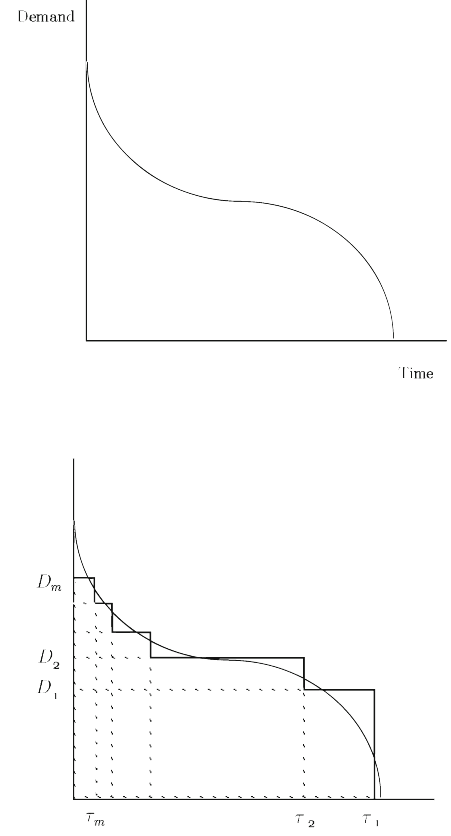
over time. Analysts usually represent the demand in terms of a so-called load dura-

tion curve that describes the demand over time in decreasing order of demand level

(Figure 5). The curve gives the time,

, that each demand level, D , is reached. Be-

cause here we are concerned with investments over the long run, the load duration

curve we consider is taken over the life cycle of the plants.

The load duration curve can be approximated by a piecewise constant curve (Fig-

ure 6) with m segments. Let d

= D

, d

= D

−D

j− 1

, j = 2,...,m represent

the additional power demanded in the so-called mode j for a duration

. To obtain

a good approximation of the load curve, it is necessary to consider large values of

m . In the static situation, the problem consists of ﬁnding the optimal investment for

each mode j , i.e., to ﬁnd the particular type of power plant i , i = 1,...,n ,that

minimizes the total cost of effectively producing 1 MW (megawatt) of electricity

during the time

.Itisgivenby

i( j)=argmin

i=1,...,n



+ q



, (3.1)

where n is the number of available technologies and argmin represents the index

i for which the minimum is achieved.

The static model (3.1) captures one essential feature of the problem, namely,

that base load demand (associated with large values of

, i.e., small indices j )

is covered by equipment with low operating costs (scaled by availability factor),

while peak-load demand (associated with small values of

, i.e., large indices j )

is covered by equipment with low investment costs (also scaled by their availabil-

ity factor). For the sake of completeness, peak-load equipment should also offer

operational ﬂexibility.

At least four elements justify considering a dynamic or multistage model for the

electricity generation investment problem:

• the long-term evolution of equipment costs;

• the long-term evolution of the load curve;

1.3 Capacity Expansion 29

Fig. 5 The load duration curve.

Fig. 6 A piecewise constant approximation of the load duration curve.

30 1 Introduction and Examples

• the appearance of new technologies;

• the obsolescence of currently available equipment.

The equipment costs are inﬂuenced by technological progress but also (and, for

some, drastically) by the evolution of fuel costs.

Of signiﬁcant importance in the evolution of demand is both the total energy

demanded (the area under the load curve) and the peak-level D

, which determines

the total capacity that should be available to cover demand. The evolution of the load

curve is determined by several factors, including the level of activity in industry,

energy savings in general, and the electricity producers’ rate policy.

The appearance of new technologies depends on the technical and commercial

success of research and development while obsolescence of available equipment

depends on past decisions and the technical lifetime of equipment. All the elements

together imply that it is no longer optimal to invest only in view of the short-term

ordering of equipment given by (3.1) but that a long-term optimal policy should be

found.

The following multistage model can be proposed. Let

• t = 1,...,H index the periods or stages;

• i = 1,...,n index the available technologies;

• j = 1,...,m index the operating modes in the load duration curve.

Also deﬁne the following:

• a

= availability factor of i ;

• L

= lifetime of i ;

• g

= existing capacity of i at time t , decided before t = 1;

• r

= unit investment cost for i at time t (assuming a ﬁxed plant life cycle for

each type i of plant);

• q

= unit production cost for i at time t ;

• d

= maximal power demanded in mode j at time t ;

•

= duration of mode j at time t .

Consider, ﬁnally, the set of decisions

• x

= new capacity made available for technology i at time t ;

• w

= total capacity of i available at time t ;

• y

= capacity of i effectively used at time t in mode j .

The electricity generation H-stage problem can be deﬁned as

min

x,y,w

∑

t=1



∑

i=1

·w

∑

i=1

∑

j= 1

·y



(3.2)

s. t. w

= w

t−1

+ x

−x

t−L

, i = 1,...,n , t = 1,...,H , (3.3)

∑

i=1

= d

, j = 1,...,m , t = 1,...,H , (3.4)

1.3 Capacity Expansion 31

∑

j= 1

≤ a

+ w

) , i = 1,...,n , t = 1,...,H , (3.5)

x,y, w ≥ 0 .

Decisions in each period t involve new capacities x

made available in each tech-

nology and capacities y

operated in each mode for each technology.

Newly decided capacities increase the total capacity w

made available, as given

by (3.3), where the equipment’s becoming obsolete after its lifetime is also consid-

ered. We assume x

= 0ift ≤ 0 , so equation (3.3) only involves newly decided

capacities.

By (3.4), the optimal operation of equipment must be chosen to meet demand

in all modes using available capacities, which by (3.5) depend on capacities g

decided before t = 1 , newly decided capacities x

, and the availability factor.

The objective function (3.2) is the sum of the investment plus maintenance costs

and operating costs. Compared to (3.1), availability factors enter constraints (3.5)

and do not need to appear in the objective function. The operating costs are exactly

the same and are based on operating decisions y

, while the investment annuities

and maintenance costs r

apply on the cumulativecapacity w

. Placing annuities on

the cumulative capacity, instead of charging the full investment cost to the decision

, simpliﬁes the treatment of end of horizon effects and is currently used in many

power generation models. It is a special case of the salvage value approach and other

period aggregations discussed in Section 10.2.

The same reasons that plead for the use of a multistage model motivate resorting

to a stochastic model. The evolution of equipment costs, particularly fuel costs, the

evolution of total demand, the date of appearance of new technologies, even the life-

time of existing equipment, can all be considered truly random. The main difference

between the stochastic model and its deterministic counterpart is in the deﬁnition of

the variables x

and w

. In particular, x

now represents the new capacity of i

decided at time t , which becomes available at time x

,where

is the con-

struction delay for equipment i . In other words, to have extra capacity available at

time t , it is necessary to decide at t −

, when less information is available on the

evolution of demand and equipment costs. This is especially important because it

would be preferable to be able to wait until the last moment to take decisions that

would have immediate impact.

Assume that each decision is now a random variable. Instead of writing an ex-

plicit dependence on the random element,

, we again use boldface notation to

denote random variables. We then have:

• x

= new capacity decided at time t for equipment i , i = 1,...,n ;

• w

= total capacity of i available and in order at time t ;

• ξ = the vector of random parameters at time t ;

and all other variables as before. The stochastic model is then

32 1 Introduction and Examples

min E

∑

t=1



∑

i=1

∑

i=1

∑

j= 1



(3.6)

s. t. w

= w

t−1

+ x

−x

t−L

, i = 1,...,n , t = 1,...,H , (3.7)

∑

i=1

= d

, j = 1,...,m , t = 1,...,H , (3.8)

∑

j= 1

≤ a

+ w

t−

) , i = 1,...,n , t = 1,...,H , (3.9)

w,x, y ≥0 ,

where the expectation is taken with respect to the random vector

ξ =(ξ

,...,ξ

) . Here, the elements forming ξ

are the demands,

,...,d

) , and the cost vectors, (r

) . In some cases, ξ

can also contain the

lifetimes L

, the delay factors

, and the availability factors a

, depending on the

elements deemed uncertain in the future.

Formulation (3.6)–(3.9) is a convenient representation of the stochastic program.

At some point, however, this representation might seem a little confusing. For ex-

ample, it seems that the expectation is taken only on the objective function, while

the constraints contain random coefﬁcients (such as d

in the right-hand side of

(3.8)).

Another important aspect is the fact that decisions taken at time t , (w

) ,are

dependent on the particular realization of the random vector, ξ

, but cannot depend

on future realizations of the random vector. This is clearly a desirable feature for a

truly stochastic decision process. If demands in several periods are high, one would

expect investors to increase capacity much more than if, for example, demands re-

main low.

Formally, if the decision variables (w

) were not dependent on ξ

, the ob-

jective function in (3.6) could be replaced by

∑



∑



∑



¯r

·w

∑



(3.10)

where ¯r

= E

and q

= E

) , making problem (3.6)to(3.9) determin-

istic. In the next section, we will make the dependence of the decision variables on

the random vector explicit.

The formulation given earlier is convenient in its allowing for both continuous

and discrete random variables. Theoretical properties such as continuity and con-

vexity can be derived for both types of variables. Solution procedures, on the other

hand, strongly differ.

Problem (3.6)to(3.9) is a multistage stochastic linear program with several

random variables that actually has an additional property, called block separable

recourse. This property stems from a separation that can be made between the

aggregate-level decisions, (x

) , and the detailed-level decisions, y

1.3 Capacity Expansion 33

We will formally deﬁne block separability in Chapter 3, but we can make an ob-

servation about its effect here. Suppose future demands are always independent of

the past. In this case, the decision on capacity to install in the future at some t only

depends on available capacity and does not depend on the outcomes up to time t .

The same x

must then be optimal for any realization of ξ . The only remaining

stochastic decision is in the operation-level vector, y

, which now depends sepa-

rately on each period’s capacity. The overall result is that a multiperiod problem

now becomes a much less complex two-period problem.

As a simple example, consider the following problem that appears in Louveaux

and Smeers [1988]. In this case, the resulting two period model has three operating

modes, n = 4 technologies,

= 1 period of construction delay, full availabilities,

a ≡1 , and no existing equipment, g ≡0 . The only random variable is d

= ξ .The

other demands are d

= 3andd

= 2 . The investment costs are r

=(10,7,16,6)

with production costs q

=(4, 4.5,3.2,5.5)

and load durations

=(10,6,1)

We also add a budget constraint to keep all investment below 120 . The resulting

two-period stochastic program is:

min 10x

+ 7x

+ 16x

+ 6x

+ E

[

∑

j= 1

(4y

1 j

+ 4.5y

2 j

+ 3.2y

3 j

+ 5.5y

4 j

)]

s. t. 10x

+ 7x

+ 16x

+ 6x

≤ 120 , (3.11)

−x

∑

j= 1

≤ 0 , i = 1,...,4 ,

∑

i=1

= ξ ,

∑

i=1

= d

, j = 2,3 ,

≥ 0 , x

≥ 0 ,

≥ 0 , i = 1,...,4 , j = 1,2, 3 .

Assuming that ξ takes on the values 3 , 5 , and 7 with probabilities 0.3, 0.4,and

0.3 , respectively, an optimal stochastic programming solution to (3.11) includes

1∗

=(2.67, 4.00,3.33,2.00)

with an optimal objective value of 381.85 . We can

again consider the expected value solution, which would substitute ξ ≡5in(3.11).

An optimal solution here (again not unique) is ¯x

=(0.00,3.00, 5.00,2.00)

.The

objective value, if this single event occurs, is 365 . However, if we use this solution

in the stochastic problem, then with probability 0.3 , demand cannot be met. This

would yield an inﬁnite value of the stochastic solution.

Inﬁnite values probably do not make sense in practice because an action can

be taken somehow to avoid total system collapse. The power company could buy

from neighboring utilities, for example, but the cost would be much higher than