Biringen S., Chow C.-Y. An Introduction to Computational Fluid Mechanics by Example

Подождите немного. Документ загружается.

162 VISCOUS FLUID FLOWS

Plot this quantity as a function of η for water, air, and mercury, and then give a

physical interpretation of the result.

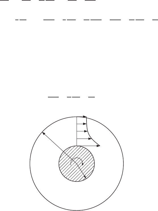
Problem 3.5 Consider a layer of ﬂuid around an inﬁnitely long circular cylin-

der of radius r

. Radial gravitational forces hold the ﬂuid in a state of static

equilibrium, forming a free surface of radius r

, as shown in Fig. 3.3.1. The ﬂuid

has a constant density ρ and viscosity coefﬁcient μ. When the cylinder is given

a rotational motion about its axis, a ﬂuid motion v

is induced in the azimuthal

direction. The θ component of the Navier-Stokes equation in cylindrical coordi-

nates is (from Hughes and Gaylord, 1964, p. 25)



∂v

∂t

∂v

∂r

∂v

∂θ

∂v

∂z



=−

∂p

∂θ

+μ



∂

∂r

∂v

∂r

∂

∂θ

∂

∂z

∂v

∂θ

−



(3.3.18)

Because of the axisymmetry of the ﬂow on the r-θ plane, derivatives with respect

to θ and z are all zero, and there are no motions in radial and axial directions.

When a steady state is reached, all terms in (3.3.18) vanish, except the ﬁrst two

and the last one in the parentheses on the right-hand side.

If the constant tangential speed at the surface of the cylinder is v

,wemay

introduce a dimensionless radial distance R = r/r

and a dimensionless speed

V = v

, so that the resultant equation becomes

−

= 0 (3.3.19)

FIGURE 3.3.1 Fluid motion around a rotating cylinder.

PIPE AND OPEN-CHANNEL FLOWS 163

The boundary conditions are, with R

representing r

V = 1atR = 1 (3.3.20)

= 0atR = R

(3.3.21)

The second condition simply states that shear stress must vanish at the free

surface. If such a stress did exist, no tangential force could be generated above

the free surface to balance it, and the equilibrium condition could never be

attained.

Divide the ﬂuid region into 50 equally spaced radial intervals and ﬁnd the

velocity distribution for R

= 2 by use of the subroutine TRID. Compute local

percent errors from the exact solution that

V =

1 + R





(3.3.22)

Notice that if a diagram similar to Fig. 2.2.1 is constructed, the ﬂuid region

should be contained between R

and R

, leaving R

n+1

as a ﬁctitious point to

handle the derivative boundary condition at the free surface.

It is interesting to see that, from (3.3.22) or the numerical result, the ﬂuid

layer will not rotate with the cylinder like a solid body under the steady state.

This result analogously explains why, even in the absence of differential solar

heating and many other factors, our atmosphere can never achieve a solid-body

rotation with the earth.

3.4 PIPE AND OPEN-CHANNEL FLOWS

With properly chosen geometries, the equations governing some viscous ﬂows

may become linearized. One example is given by Problem 3.5 in the preceding

section; it concerns the angular motion of ﬂuid between two concentric circles.

In this section a class of ﬂows is considered whose governing equation is linear

but involves two independent variables.

We consider the general problem of steady incompressible ﬂow through a

straight pipe of uniform but arbitrary cross section. The ﬂow may be caused

by either an applied pressure gradient, the gravitational force, the motion of a

part of the pipe wall relative to the rest, or any combination of these factors.

The ﬂow may be enclosed by a rigid wall or it may have a free surface. More-

over, the ﬂow may contain multiply connected regions formed by axial inner

tubes.

Let the inﬁnitely long pipe be parallel to the x-axis along which ∂V/∂x = 0.

Because of this particular geometry, the ﬂow has only one nonvanishing velocity

component u in the axial direction, so that the continuity equation (3.1.6) is

satisﬁed automatically and the nonlinear terms on the left side of momentum

164 VISCOUS FLUID FLOWS

equation (3.1.7) disappear. There is only one equation governing u of the form

∂

∂y

∂

∂z



−f



(3.4.1)

where the x component of the gravitational force per unit volume, f

, has been

added. It turns out that we have a Poisson equation to which the iteration methods

developed in Section 2.8 apply.

If f

= 0 and the pipe cross section is circular, (3.4.1) describes the classi-

cal problem of the Poiseuille ﬂow, whose analytical solution can be obtained

immediately. Although (3.4.1) is a linear equation, to ﬁnd its analytical solution

satisfying a set of arbitrary boundary conditions is still a difﬁcult task. Numeri-

cal solution of (3.4.1) is generally required except for a few cases in which the

cross-sectional shape can be described by some simple geometries.

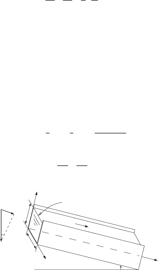
As an illustrative example for solving this class of problems, we consider a

tilted open channel of square cross section making an angle θ with the horizontal

(Fig. 3.4.1). The x axis is still chosen to be parallel to the channel, and the angle θ

is assumed to be so small that the free surface is everywhere parallel to the chan-

nel base. Since there is no applied pressure gradient along the channel, the only

forcing function on the right side of (3.4.1) is that due to f

= ρg sin θ, g being

the gravitational acceleration. With the introduction of dimensionless variables

Y =

, Z =

, U =

ρg sin θ/μ

(3.4.2)

where L is the width or height of the square cross section, (3.4.1) becomes

∂

∂Y

∂

∂Z

=−1 (3.4.3)

sin θ

ρg

Horizontal line

Free Surface

FIGURE 3.4.1 An open-channel ﬂow.

PIPE AND OPEN-CHANNEL FLOWS 165

Boundary conditions require that velocity vanishes at solid walls and shear stress

is zero at the free surface, or, mathematically,

U = 0atY = 0andatZ = 0 and 1 (3.4.4)

∂U

∂Y

= 0atY = 1 (3.4.5)

For a numerical solution a square grid system is set up to cover the region

occupied by the ﬂuid in the Y -Z plane. With the grid size h = 0.05, we obtain

21 (= m) vertical grid lines and 21 (= n) horizontal grid lines. Because of the

derivative boundary condition (3.4.5), a ﬁctitious horizontal line is needed at

a distance h above the free surface. Comparing (3.4.3) with the generalized

form (2.8.1) of the Poisson equation, we can write down its ﬁnite-difference

computational scheme based on the successive overrelaxation formula (2.8.13):

i, j

= (1 −ω)U

i, j



i−1,j

i+1,j

i,j−1

i,j+1



(3.4.6)

Here the superscripts used in (2.8.13) to indicate the number of iterations are

omitted; they are not needed if in each iteration (3.4.6) is applied successively at

interior points starting from the lower left corner of the grid. The optimum value

for the relaxation parameter ω is determined according to (2.8.14).

In index notation the boundary conditions (3.4.4) become

i,1

= 0, i = 1, 2, ..., m (3.4.7)

1, j

= U

m, j

= 0, j = 1, 2, ..., n (3.4.8)

After replacing the derivative in (3.4.5) by its central-difference approximation,

the derivative boundary condition is reduced to

i, n+1

= U

i, n−1

, i = 2, 3, ..., m − 1 (3.4.9)

In the program to follow the conditions (3.4.7) and (3.4.8) are assigned at the

beginning and are kept the same for all iterations, while (3.4.9) is used in the

computation of (3.4.6) in every iteration whenever j reaches the value n.

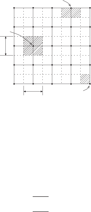
Knowing the velocity distribution across a section, we can calculate the vol-

ume of ﬂuid passing through the channel per unit time. Let the solid lines in

Fig. 3.4.2 represent schematically the grid system covering the channel cross

section. Dashed vertical and horizontal lines are then drawn to bisect the solid-

line square meshes.

At each of the grid points marked at the intersections of solid lines, the dimen-

sionless velocity U is either given or computed. These points may be grouped

into three categories according to their locations: the interior points, the bound-

ary points, and the corner points, as indicated in Fig. 3.4.2. For small mesh sizes

we may assume that the velocity in the shaded area containing a grid point is

approximately the same as that at the point itself. As shown in the ﬁgure, the

shaded small area for an interior point is of magnitude h

, that for a boundary

166 VISCOUS FLUID FLOWS

Boundary Point

Corner Point

Interior

Point

FIGURE 3.4.2 Evaluation of volume ﬂow rate.

point is h

/2, and that for a corner point is h

/4. The volume ﬂow rate is cal-

culated approximately by summing the products of local velocity and area at all

grid points.

In the output of Program 3.3 some of the numerical values of U are tabulated

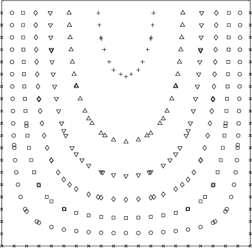
(Table 3.A.3) and, in addition, velocity contours are plotted in Fig. 3.4.3. Variables

used in this program are named according to their original forms; the name

VOLRAT is used for the volume ﬂow rate.

The result shows that the maximum velocity occurs at the middle of the free

surface having the magnitude 0.114 L

ρg sin θ/μ, and the volume ﬂow rate is

0.0569 L

ρg sin θ/μ. It is interesting to compare this result with the analytical

result obtained for the same free-surface ﬂow with the two side walls removed.

The velocity proﬁle and volume ﬂow rate in such a channel of width L are, from

Batchelor (1967, p. 183), expressed in our notation,

u =

ρg sin θ

2μ

y(2L −y) (3.4.10)

Q =

ρg sin θ

3μ

(3.4.11)

The maximum velocity at the free surface is then 0.5 L

ρg sin θ/μ,whichis

4.4 times the value in the presence of two side walls separated by a distance

equal to the ﬂuid depth, and the ﬂow rate becomes 5 times bigger. The compar-

ison reveals that the side walls have a tremendous retardative effect on channel

ﬂows.

PIPE AND OPEN-CHANNEL FLOWS 167

FIGURE 3.4.3 Velocity distribution across an open channel of square cross section. ×,

U = 0;

◦

, U = 0.018; , U = 0.036; ♦, U = 0.054; ∇, U = 0.072; , U = 0.09; +, U = 0.108.

Problem 3.6 Consider a channel with a square cross section of area L

having

a movable upper wall. Find the velocity distribution and the volume ﬂow rate of

the steady ﬂow caused by moving the upper wall at a constant velocity u

in the

direction parallel to the channel length.

Assume that the gaps between the moving and the stationary side walls are

smaller than the grid width h. The boundary condition on the uppermost grid

line is that the velocity is u

at all grid points except those at the corners, where

the velocity is zero.

Problem 3.7 Solve the problem in which the upper movable wall described in

Problem 3.6 is replaced by one of width L/2, leaving the uncovered portion of

the leveled upper ﬂuid surface free. Study the variation of ﬂow rate with the

horizontal position of the upper plate whose axial velocity is kept at the same

value u

Project for Further Study: A steady ﬂow is established in a long pipe after a

constant pressure gradient dp/dx has been applied along the axis for a long time.

Compute the velocity distribution and the volume ﬂow rate of an incompressible

ﬂuid in pipes of the cross-sectional shapes described in Fig. 3.4.4.

168 VISCOUS FLUID FLOWS

(a)(b)(c)

= 0 45°

45°

= 0

∂u

∂z

∂u

∂y

FIGURE 3.4.4 Various tube cross sections.

1. A circular tube of radius R. From symmetry only the ﬁrst quadrant is

needed for the numerical computation. The boundary conditions at the two

straight edges of the fan-shaped domain are that the variations of velocity

normal to the edges are zero. To handle the curved boundary, the method

of Program 2.7 may be used.

Compare the numerical result with the analytical solution for Poiseuille

ﬂow (Batchelor, 1967, p. 180) that

u =−

4μ



−r



Q =−

πR

8μ

2. A triangular tube whose two slant walls make 45

◦

angles with the third.

3. A rectangular tube containing a square inner tube.

3.5 EXPLICIT METHODS FOR SOLVING PARABOLIC

PARTIAL DIFFERENTIAL EQUATIONS—GENERALIZED

RAYLEIGH PROBLEM

In studying the development of a boundary layer on a body moving through

an incompressible ﬂuid, Rayleigh (1911) considered the unsteady motion of an

inﬁnitely extended ﬂuid in response to an inﬁnite ﬂat plate suddenly set in motion

along its own plane. If the plate is normal to the y axis and the motion is in

the x direction, the continuity equation (3.1.6) is satisﬁed automatically and the

incompressible Navier-Stokes equation (3.1.7) is simpliﬁed to

∂u

∂t

= ν

∂

∂y

(3.5.1)

EXPLICIT METHODS FOR SOLVING PARABOLIC PARTIAL DIFFERENTIAL EQUATIONS 169

Sometimes this equation, governing arbitrary unsteady planar ﬂuid motions, is

expressed in terms of vorticity ζ(=−∂u/∂y) in the form

∂ζ

∂t

= ν

∂

∂y

(3.5.2)

which describes the diffusion of vorticity through a one-dimensional space.

According to the discussions of Section 2.7, both (3.5.1) and (3.5.2) are classi-

ﬁed as parabolic partial differential equations. Here we will construct a numerical

scheme for solving (3.5.1), examine its computational stability, and then apply it

to a particular physical problem.

In numerical computations the space coordinates must be ﬁnite. Let us assume

that the ﬂuid above the plate at y = 0 is bounded below a ﬁnite depth that

is divided into m − 1 equally spaced intervals of size h. If the time axis is

divided into steps of size τ , a grid system is formed, as shown in Fig. 3.5.1.

To approximate (3.5.1) by a ﬁnite difference equation at the grid point (i, j),

the second-order spatial derivative is replaced by the central-difference formula

(2.2.9) and the time derivative is replaced by the forward-difference formula

(2.2.6). After rearrangement the equation has the ﬁnal form

i, j +1

= u

i, j

+R(u

i−1, j

−2u

i, j

i+1, j

) (3.5.3)

in which R = ντ/h

is a dimensionless parameter. The equation states that the

solution at a certain height at time interval τ later can be computed based on the

present information at the local and two neighboring stations. For given boundary

conditions expressed as known functions of time, the solution at time level t

computed explicitly from the initial condition at t

by using (3.5.3). Repeating

the procedure for the successive time steps, the solution at any desired time level

can be obtained. For this property the method in which (3.5.3) is applied is called

an explicit method for solving the parabolic equation (3.5.1).

Playing a similar role as the Courant number C in (2.10.4), the parameter R in

(3.5.3) cannot be arbitrarily chosen, and the limitation imposed on its magnitude

(i + 1, j )

(i − 1, j )

(i, j )

(i, j + 1)

FIGURE 3.5.1 An explicit method for solving parabolic equations.

170 VISCOUS FLUID FLOWS

is to be determined from a stability analysis of the numerical scheme. Following

the technique illustrated in Section 2.10, we assume

i, j

= U

Iikh

(3.5.4)

and obtain, after substituting into (3.5.3),

j+1

= [1 −2R(1 −cos kh)]U

(3.5.5)

The quantity contained within the brackets is the ampliﬁcation factor λ.If|λ|> 1,

j+1

|> |U

| and the amplitude of the solution becomes unbounded as j →∞.

This is called an unstable situation. Thus, for stability we require λ

≤ 1or,

consequently, after expanding the left-hand side,

R ≤

1 − cos kh

Since the lowest value of the expression on the right-hand side is 1/2 when

cos kh =−1, the stability criterion derived for (3.5.3) is

ντ

≤

(3.5.6)

When the upper limiting value is used for this parameter, (3.5.3) has a partic-

ularly simple form:

i, j +1

i−1, j

i+1, j

) (3.5.7)

This is called the Bender-Schmidt recurrence equation, which determines the

solution at (y

, t

j+1

) as the average of the values right and left of y

at a time t

However, more accurate results are obtained by using (3.5.3) for R < 1/2.

The differential equation (3.5.1) and its ﬁnite-difference approximation (3.5.3)

apply to any unsteady planar ﬂows bounded by two parallel inﬁnite plates per-

forming arbitrary parallel motions along their own planes. One of the plates may

be replaced by a free surface. Furthermore, with modiﬁcations to suit cylindrical

coordinates, the resulting equations apply to ﬂows between concentric cylinders.

Solving for the velocity and the related ﬁelds of these ﬂows may be classiﬁed as

the generalized Rayleigh problem.

For illustrative purposes we consider water contained between two originally

stationary ﬂat plates separated by a distance of 1 m. At an initial instant t = 0,

the upper plate has suddenly acquired a constant speed u

(= 1m/s) while the

lower plate is kept stationary all the time. The sudden motion of the upper plate

creates a sharp velocity change there, forming a concentrated vortex sheet right

below the plate. The vorticity is diffused downward, according to (3.5.2), into

EXPLICIT METHODS FOR SOLVING PARABOLIC PARTIAL DIFFERENTIAL EQUATIONS 171

a region practically free of vorticity, and the velocity is redistributed accord-

ingly. We like to ﬁnd numerically the velocity distribution across the channel at

different times.

In terms of the notation of Fig. 3.5.1, the initial velocity distribution is

i,1

= 0for1= 1, 2, ..., m −1

m,1

= u

and the boundary conditions are

1, j

= 0 for j > 1

m, j

= u

for j > 1

For water ν = 1 ×10

−6

/s, approximately. If the space between plates is

divided into 20 equal intervals, then m = 21 and h = 0.05 m. Let us choose

R = 1/4, which determines the time interval τ = Rh

/ν or 625 s. This time step

size seems to be rather large. But it is a reasonable size for a laminar shear

ﬂow in which vorticity or velocity gradient is diffused purely by intermolecular

activities characterized by a small kinematic viscosity.

In the form shown in (3.5.3), the velocity ﬁeld is a two-dimensional array. This

is not necessary, however, in programming for the computation. In Program 3.4

we use one-dimensional arrays

UOLD(I) and UNEW(I) to denote u

i, j

and u

i, j +1

respectively and overwrite them at successive time steps for efﬁcient use of

computer memory. The solution for U is shown in Fig. 3.5.2 for the ﬁrst ﬁve

curves.

The output (Table 3.A.4) shows that a velocity discontinuity cannot exist in

a viscous ﬂuid and is smoothed out immediately by viscous diffusion. As time

progresses the velocity proﬁle approaches a linear distribution that varies from 0

at the lower plate to 1 m/s at the upper and corresponds to the solution for the

Couette ﬂow between two parallel plates in a steady shear motion.

Problem 3.8 Assign a value to R that is greater than 0.5, and then run Program

3.4 to watch the growth of the solution to some unrealistic magnitudes. The result

proves the validity of the stability criterion (3.5.6).

Problem 3.9 Find the velocity distribution at increasing times in the originally

stationary ﬂuid around a circular cylinder with a free surface (Fig. 3.3.1) after

the cylinder is suddenly given a rotation of tangential speed v

at the surface.

As time approaches a very large value, the solution should approach that for

Problem 3.6.