Blank B.E., Krantz S.G. Calculus: Single Variable

Подождите немного. Документ загружается.

and

ðTÞ5



ðα=2 2 1Þβ 2 T



ðT 1 βÞ

EðTÞ:

Deduce that E is an increasing function of T with a sig-

moidal (or S-shaped) graph. What is the point of inﬂec-

tion of the graph of E?

92. Suppose that h

, k,andq are positive constants with q , 1.

Show that the Chapman-Richards function, deﬁned by

hðtÞ5 h





1 2 expð2qktÞ



1=q

;

is the solution of the initial value problem

ðtÞ5 k  hðtÞ



hðtÞ



2 1



; hð0Þ5 0;

which is used in forest management to model tree growth.

Here t represents time, and h measures tree height (or

some other growth indicator).

Calculator/Computer Exercises

c In each of Exercises 93296, solve the given initial value

problem for y(x). Determine the value of y(2). b

93. dy/dx 5 (1 1 x

) /(1 1 y

) y(0) 5 0

94. dy/dx 5 (x

) /(1 1 sin( y)) y(0) 5 0

95. y

dy/dx 5 (1 1 y)/(1 1 2x) y(0) 5 0

96. dy/dx 5 x/(1 1 e

) y(0) 5 0

97. The weight y of a goose is determined as a function of

time by the initial value problem dy=dt 5 0:09 

ﬃﬃ

ð5000 2 yÞ; yð0Þ5 175 when t is measured in weeks

after birth, and y is measured in grams. In how many

weeks does the goose reach half of its mature weight?

98. Suppose that in a certain ecosystem, x 100 denotes the

number of predators, and y 1000 denotes the number of

prey. Suppose further that the relationship between the

two population sizes satisﬁes the following Lotka-

Volterra equation:

y ð6 2 2xÞ

x ð4y 2 5Þ

Separate variables, and solve this equation. If the initial

prey population is 1500, and the initial predator popula-

tion is 200, what are the possible sizes of the population of

prey when the predator size is 300?

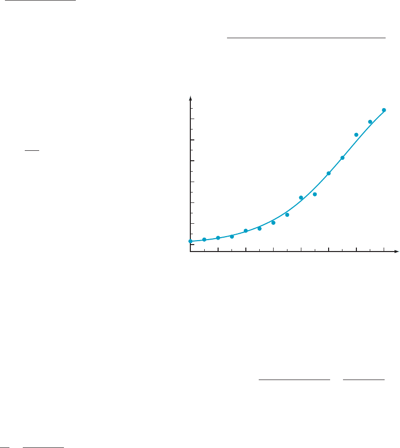
99. As the result of pollution reduction in the Great Lakes

region, certain species of wildlife that had been

threatened have made a comeback. Figure 13 contains a

plot of the number P of double-crested cormorant nests in

the Great Lakes region for the years 1979 through 1993.

A logistic growth curve has been superimposed. In this

exercise, you will obtain the formula for the logistic curve

PðtÞ5

 P

1 ðP

2 P

Þexp



2k  P

ðt 2 1979Þ



Use P

5 44000 for the carrying capacity, and use P

P(1979) 5 800 for the value of the initial population.

a. For t 5 1984, 1985, ..., 1988, use a central difference

quotient to approximate P

(t). For example,

ð1980Þ

Pð1981Þ2 Pð1979Þ

1981 2 1979

1600 2 800

The logistic differential equation P

(t) 5 kP(t)(P

P(t)) then permits an estimate for k. Average the ﬁve

estimates to get a working value of k.

b. Using the value of k obtained in part a, calculate P(t)

for t 5 1990, ...,1993. (Although the observed values

for these years appear in Figure 13, they were not used

to obtain the model. Comparing the predicted values

with the observed values is a reality check for the

model.)

c. Plot the logistic growth curve for 1979 # t # 1993.

d. According to your logistic model, about when did the

number of nests reach 43,000?

1993

800

1200

1600

3300

1900

19811979 1983

3800

5200

7100

12000

17000

20700

26200

29300

32100

11200

1985 1987 19911989

10000

5000

15000

20000

25000

30000

m Figure 13 Cormorant nests (19791993)

7.6 First Order Differential Equations—Separable Equations 605

7.7 First Order Differential Equations—Linear Equations

In the preceding section, you learned a method for solving the ﬁrst order differ-

ential equation

5 Fðx; yÞ

when F(x, y) 5 g(x)  h( y). There are several other methods that are similarly

adapted to other particular forms assumed by F(x, y). In this section, we will study

the case in which F(x, y) 5 q(x) 2 p(x) y.

Solving Linear

Differential Equations

We say that a ﬁrst order differential equation of the form

5 qðxÞ2 pðxÞy

is linear. We often write a linear equation in the standard form

1 pðxÞy 5 qðxÞ: ð7: 7 :1Þ

This algebraic step does not separate variables, but it does eliminate the y variable

from the right side of the equation, and it prepares the left side for multiplication

by an “integrating factor” followed by a decisive application of the Product Rule

for differentiation.

THEOREM 1

Suppose that p(x ) and q(x) are continuous functions. Let P(x)be

any antiderivative of p(x). Then the general solution of the linear equation

1 pðxÞy 5 qðxÞ

yðxÞ5 e

2PðxÞ

PðxÞ

qðxÞdx 1 Ce

2PðxÞ

; ð7:7:2Þ

where C is an arbitrary constant.

Proof. The

presence of both y

(x) and y(x) in the sum on the left side of equation

(7.7.1) leads us to consider the Product Rule for differentiation. If u is a function of

x that is never 0, then we have

ðuyÞ5 u





y 5 u





The idea is to ﬁnd a function u so that the factor of y on the right side of the

preceding equation matches the factor of y in (7.7.1). That is, we want to ﬁnd a

function u such that

uðxÞ





5 pðxÞ:

606 Chapter 7 Applications of the Integral

As we learned in Section 7.6, we solve this separable differential equation by

rewriting it as

du 5

pðxÞdx:

Because P(x) is an antiderivative of p(x), the general solution of the preceding

equation is ln(|u|) 5 P(x) 1 C

, where C

is a constant of integration. Because any

particular solution u will serve our purpose, we simplify the algebra by choosing a

solution u with u(x) . 0andC

5 0. With these choices, we have ln(u) 5 P(x), or

u(x) 5 e

P(x)

. This is our integrat ing factor. On multiplying each side of equation

(7.7.1) by e

P(x)

, we obtain

pðxÞe

PðxÞ

 y 1 e

PðxÞ

5 e

PðxÞ

qðxÞ:

Thus



PðxÞ

 y





PðxÞ



 y 1 e

PðxÞ

5 P

ðxÞe

PðxÞ

 y 1 e

PðxÞ

5 pðxÞe

PðxÞ

 y 1 e

PðxÞ

5 e

PðxÞ

qðxÞ:

In other words, e

P(x)

 y is an antiderivative of e

P(x)

q(x). That is,

PðxÞ

 y 5

PðxÞ

qðxÞdx 1 C;

from which formula (7.7.2) is obtained on divi ding each side by e

P(x)

. ’

⁄ EXAMPLE 1 Solve the initial value problem

5 4x; yð2Þ5 3:

Solution The

given differential equation is linear: It has the form of equation

(7.7.1) with p(x) 5 2/x and q(x) 5 4x. Because

pðxÞdx 5

dx 5 2lnðjxjÞ1 C;

and because we may choose any antiderivative of p(x)forP(x), we set P(x) 5 2ln(|x|).

We note from the initial condition that the positive number 2 must belong to the

interval on which the required solution y(x) is deﬁned. This interval of deﬁnition

cannot contain any negative number because, if it did, then 0 would be in the interval.

However, we see that the differential equation is not even deﬁned when x 5 0, so it

cannot hold when x 5 0. Thus the domain of deﬁnition of y is limited to positive values.

We may therefore dispense with the absolute value function and take P(x) 5 2ln(x).

Thus

PðxÞ

5 e

2lnðxÞ

5 e

lnðx

5 x

and equation (7.7.2) become

yðxÞ5 x

 4xdx1 C  x

dx 1



5 x

Because y(2) 5 2

1 C/2

5 4 1 C/4, the initial condition tells us that 4 1 C/4 5 3. It

follows that C 524, and y(x) 5 x

2 4/x

. ¥

7.7 First Order Differential Equations—Linear Equations 607

⁄ EXAMPLE 2 Solve the initial value problem

1 y 5 sinðxÞ; yðπ=2Þ5 2:

Solution To

put this equation into the form of equation (7.7.1), we divide by x and

obtain

 y 5

sinðxÞ

We set p(x) 5 1/x, q(x) 5 sin(x)/x , and take P( x ) 5 ln(x) for an antiderivative of

p(x). (The reasoning for taking ln(x) instead of ln(|x|) 1 C is similar to that

of Example 1.) It follows that e

P(x)

5 e

ln(x)

5 x and equation (7.7.2) become

yðxÞ5 x

x 

sinðxÞ

dx 1 C  x

sinðxÞdx 1

C 2 cosðxÞ

Because y(π/2) 5 2, we have

C 2 cosðπ=2Þ

π=2

5 2;

or C 5 π. Thus

yðxÞ5

π 2 cosðxÞ

: ¥¥

⁄ EX

AMPLE 3 Find the general solution of the linear differential equation

1 tanðxÞy 5 secðxÞ



0 , x ,



Do not use equation (7.7.2). Instead, use the technique found in the proof of

Theorem 1.

Solution We

recall that ln(sec(x)) is an antid erivative of tan(x). In the notation of

Theorem 1, q(x) 5 sec(x), p(x) 5 tan(x), and P(x) 5 ln(sec(x)). We multiply each side

of the given differential equation by e

P(x)

. Observing that e

P(x)

5 e

ln(sec(x))

5 sec(x),

we obtain

secðxÞ tanðxÞy 1 secðxÞ

5 sec

ðxÞ;



secðxÞ



 y 1 secðxÞ

5 sec

ðxÞ;



secðxÞy



5 sec

ðxÞ:

It follows that

secðxÞy 5

sec

ðxÞdx 5 tanðxÞ1 C;

608 Chapter 7 Applications of the Integral

y 5

tanðxÞ

secðxÞ

5 sinðxÞ1 C cos ðxÞ: ¥¥

An Application: Mixing

Problems

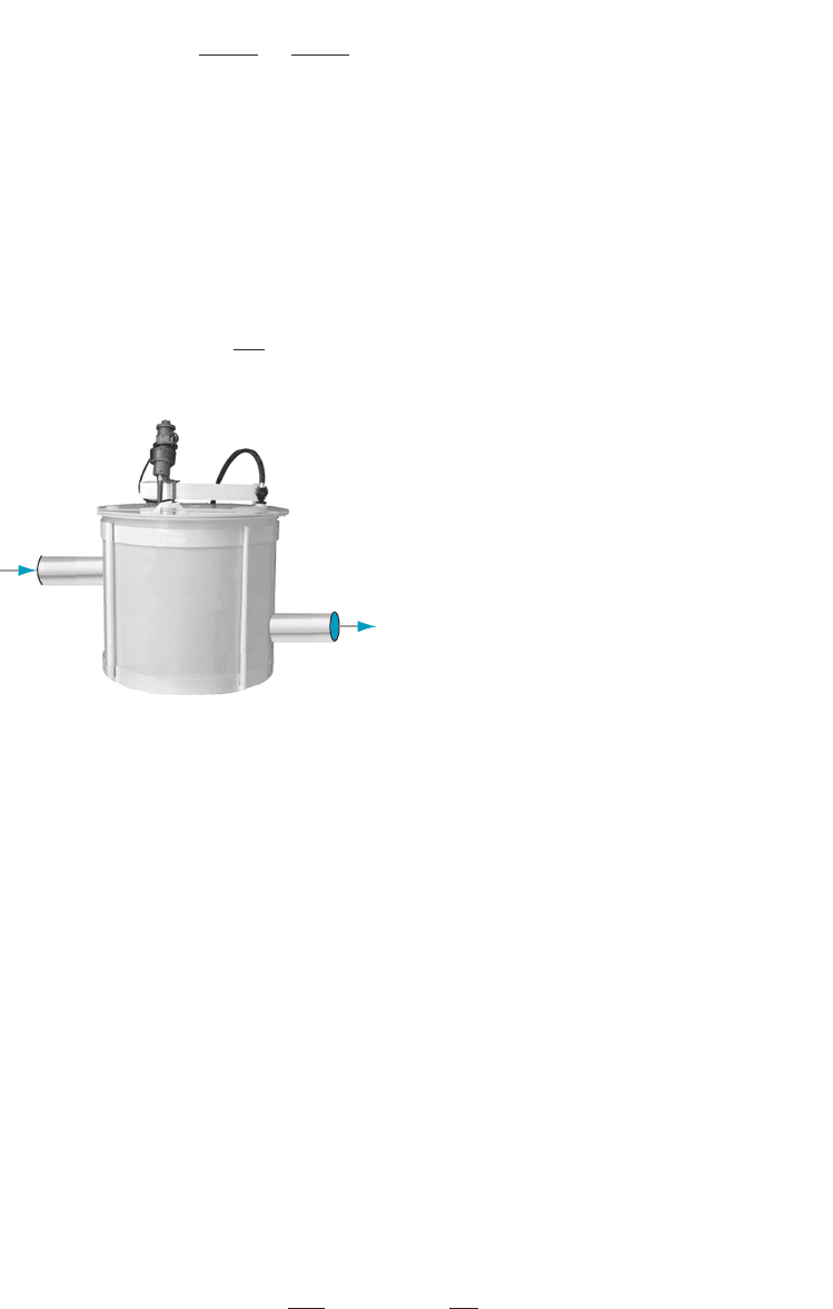
Mixing problems occur frequently in biology, chemistry, medicine, and pharma-

cology. In a basic mixing problem, a container contains a substance in solution.

There is an inlet to the co ntainer as well as an outlet (see Figure 1). When ﬂuid

enters and exits the tank through these channels, the solution in the tank can

become enriched or diluted. If m is the mass of the dissolved sub stance, then the

basic equation becomes

5 ðrate inÞ 2 ðrate outÞ: ð7:7:3Þ

To apply the theory of linear equations, we must assume that the solution is

thoroughly mixed at all times so that the concentration of the solution is homo-

geneous throughout the container. (Nearly all mathematical models involve some

approximation. Many involve a compromise between accuracy and simplicity. A

completely accurate model that is too difﬁcult to solve may do us little good. By

simplifying the model somewhat, we may be able to obtain a useful solution

without sacriﬁcing too much accuracy.)

⁄ EX

AMPLE 4 A 200 gallon tank is ﬁlled with a salt solution initially con-

taining 10 pounds of salt. An inlet p ipe brings in a solu tion of salt at the rate of 10

gallons per minute. The concentratio n of salt in the incoming solution is 1 2 e

2t/60

pounds per gallon when t is measured in minutes. An outlet pipe prevents overﬂow by

allowing 10 gallons per minute to ﬂow out of the tank. How many pounds of salt are in

the tank at time t? Long term, about how many pounds of salt will be in the tank?

Solution Let m(t)

be the amount of salt in the tank at time t. To calculate the

amounts of salt entering the tank through one pipe and exiting through another, we

multiply the rate at which the ﬂuid enters and exits by the appropriate

concentrations. The rate at which salt enters the tank is

gal

min

ð1 2 e

2t=60

gal

;

Fluid in

ACME

Fluid out

-210

-190

170

-150

130

-110

-90

-70

-50

m Figure 1

7.7 First Order Differential Equations—Linear Equations 609

or 10 ð1 2 e

2t=60

Þ pounds per min ute. The rate at which salt leaves the tank is

gal

min



200

gal

;

or m/20 pounds per minute. Equation (7.7.3) becomes

5 10 



1 2 e

2t=60



;

m 5 10 



1 2 e

2t=60



;

which is a linear differential equation. Of course, the use of t rather than x as an

independent variable does not affect the applicability of Theorem 1. We simply use

t instead of x and set p(t) 5 1/20 and q(t) 5 10(1 2 e

2t/60

). Then P(t) 5 t/20 and

equation (7.7.2) gives us

mðt Þ5 e

2t=20

t=20



1 2 e

2t=60



dt 1 Ce

2t=20

5 10 e

2t=20



t=20

2 e

t=30



dt 1 Ce

2t=20

;

mðtÞ5 100



2 2 3e

2t=60



1 Ce

2t=20

Because m(0) 5 10, we have 10(20 2 30e

20/60

) 1 Ce

20/20

5 10, or 10(20 2 30) 1

C 5 10, or C 5 110. Thus

mðt Þ5 100



2 2 3e

2t=60



1 110e

2t=20

Notice that

lim

t-N



100



2 2 3e

2t=60



1 110e

2t=20





100ð2 2 3  0Þ1 110  0



5 200:

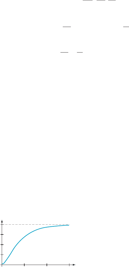
Thus the amount of salt in the tank approaches 200 pounds. Figure 2 plots the

increasing quantity of salt for the ﬁrst ﬁve hours of the process.

An Application:

Electric Circuits

Figure 3 is the schematic diagram of a simple electric circuit involving an elec-

tromotive force of E(t) volts (such as produced by a battery or a generator), a

resistor with a resistance of R ohms (Ω), and an inductor with inductance of L

200

150

100

y  200

0 200 300

(

minutes

)

m(t)  100(2 3e

t/60

)110e

t/20

m Figure 2

610 Chapter

7 Applications of the Integral

henrys (h). It is a consequence of Kirchhoff’s voltage law that the current I

(measured in amperes) satisﬁes

1 R  I 5 EðtÞ:

⁄ EX

AMPLE 5 In the circuit of Figure 3, what is I(t)ifL 5 3 h, R 5 6 Ω,and

E(t) 5 12 cos(2t)V?

Solution After

dividing by L and substituting the given values, we obtain

1 2  I 5 4 cosð2tÞ:

In the notation of Theorem 1 (with I an d t taking the roles of y and x, respectively),

we have q(t) 5 4 cos(2t), p(t) 5 2, P(t) 5 2t, and e

P(t)

5 e

. Theorem 1 tells us that

the integral

PðtÞ

qðtÞdt 5

cosð2tÞdt

arises in the solution. To evaluate this integral, we make the substitution x 5 2t,

dx 5 2dt, which, by Example 5 of Section 6.1 in Chapter 6, results in

cosðxÞdx; or



sinðxÞ1 cosðxÞ



1 C. On resubstituting, we obtain

PðtÞ

qðtÞdt 5

cosð2tÞdt 5



sinð2tÞ1 cosð2tÞ



1 C:

Equation (7.7.2) of Theorem 1 then gives us

IðtÞ5 e

2PðtÞ

PðtÞ

qðtÞdt 1 Ce

2PðtÞ

5 4e

22t

cosð2tÞdt 1 Ce

22t

5 cosð2tÞ1 sinð2tÞ1 Ce

22t

: ¥

Linear Equations with

Constant Coefﬁcients

Linear equations with constant coefﬁcients arise frequen tly in applications. These

differential equations have the form dy/dt 1 βy 5 α. By rewriting this equation in

the form dy/dt 5 α 2 βy, we see that it is a separable differential equation (in

addition to being linear). Although we may solve it by using the techniques we

learned in Section 7.6, we will simplify the calculation by appealing to Theorem 1.

THEOREM 2

Suppose that α and β are constants with β 6¼0. Then the linear

differential equation

1 βy 5 α ð7:7:4Þ

has general solution

yðtÞ5

1 Ce

2βt

: ð7:7:5Þ

The initial value pro blem

1 β y 5 α; yð0Þ5 y

ð7:7:6Þ

has unique solution

yðtÞ5





2βt

: ð7:7 :7Þ

m Figure 3

7.7 First Order Differential Equations—Linear Equations 611

Proof. Equation (7.7.4) is the special case of equation (7.7.1) that results from

setting q(t) 5 α and p(t) 5 β. Because P(t) 5 βt is an antiderivative of p(t), equation

(7.7.2) tells us that equation (7.7.4) has solution

yðtÞ5 e

2βt

βt

α dx 1 Ce

2βt

1 Ce

2βt

;

which establishes equation (7.7.5). If y(0) 5 y

, then α/β 1 Ce

2β 0

5 y

,or

C 5 y

2 α/β. Substituting this formula for C into equation (7.7.5) results in

formula (7.7.7). ’

We will illustrate Theorem 2 with several different applications. In a text book,

is useful to quote formulas such as (7.7.5) and (7.7.7) to avoid consecutive

repetitions of what would be essentially the same calculation. Nevertheless, a

student will ﬁnd it more useful to understand the general technique of solving

equation (7.7.4) than to memorize the actual solution. Many equations and for-

mulas appear in calculus textbooks. The study of calculus is simpliﬁed by mastering

the basic ones and learning the techniques that treat the variants.

Newton’s Law for

Temperature Change

Suppose that T is the temperature of an object that is surrounded by a body (e.g.,

water, air, etc.) at const ant temperature T

—the reason for using this subscript will

become apparent. Newton’s Law states that the rate of change of T is proportional

to the difference between T and T

. That is,

5 k ðT

2 TÞ; ð7:7:8Þ

where the co nstant of proportionality, k, is positive. Note that if T (t) , T

, then the

right side of equation (7.7.8) is positive and therefore 0 , T

(t). As a result, T(t)

increases, and we refer to Newton’s Law of Heating. If, instead, T

, T(t), then

(t) , 0 and T decreases. In this case, we refer to Newton’s Law of Cooling.

THEOREM 3

Suppose that T

5 T(0) is the temperature of an object when it is

placed in an environment that has constant temperature T

. Suppos e that the

temperature T(t) of the object is governed by Newton’s law of temperature

change. That is, suppose that T(t) is a solution of equation (7.7.8). Then

TðtÞ5 T

1 ðT

2 T

Þe

2kt

ð0 # t , NÞ: ð7:7:9Þ

Proof. The

right side of equation (7.7.8) can be rew ritten as k T

2 k T,or

α 2 βT with α 5 k T

and β 5 k. With these values of α and β, equation (7.7.8)

becomes

1 βT 5 α:

Formula (7.7.7) gives a formula for the unique solution of the initial value problem:

TðtÞ5





2βt

kT



kT



2kt

5 T

1 ðT

2 T

Þe

2kt

: ’

612 Chapter 7 Applications of the Integral

Notice that e

2kt

-0ast-N and therefore

lim

t-N

TðtÞ5 lim

t-N



1 ðT

2 T

Þe

2kt



5 T

1 ðT

2 T

Þ lim

t-N

2kt

5 T

1 ðT

2 T

Þ 05 T

Thus as t-N, the temperature of the object approaches the ambient temperature

⁄ EX

AMPLE 6 A thermometer is at room temperature (20.0



C). One min-

ute after being placed in a patient’s throat, it reads 38.0



C. One minute later, it



C. Is this second reading an accurate measure (to three signiﬁcant digits)

of the patient’s temperature?

Solution Let T(t)

denote the temperature of the thermometer at time t with t 5 0

corresponding to the moment it is placed in the patient’s throat. Let T

denote the

actual temperature of the patient. Then,

TðtÞ5 T

1 ðT

2 T

Þe

2kt

with T

5 20. Although there are two unknowns (k and T

) in this problem, we are

given two observations with which to determine them :

38 5 Tð1Þ5 T

1 ð20 2 T

Þe

and

38:3 5 Tð2Þ5 T

1 ð20 2 T

Þe

22k

: ð7:7:10 Þ

The ﬁrst of these eq uations may be written as

38 2 T

20 2 T

5 e

: ð7:7:11Þ

Because e

22k

equals (e

)

, we may replace e

22k

in equation (7.7.10) with the

square of the left side of (7.7.11). The result is

38:3 5 T

1 ð20 2 T



38 2 T

20 2 T



This equation simpliﬁes to a linear equation in the unknown T

, which we solve to

ﬁnd T

5 38.305 . . . . The reading at t 5 2 is therefore an accurate meas ure of the

patient’s temperature to three signiﬁcant digits.

INSIGHT

In Example 6, we may calculate e

5 0.016662 . . . from equation (7.7.11)

and the previously calculated T

5 38.305. When we substitute the values of T

, T

, and

into equation (7.7.9), we ﬁnd that T( t) 5 38.305 2 18.305 (0.016662)

. The graph of

T(t) in the window [0, 2] 3 [30, 40] (see Figure 4a) indicates that T(t) is very close to T

after t 5 1.3. A closer look using the window [1.5, 2.5] 3 [38.266, 38.305] reveals that T(t)

does continue to increase, but very slowly (Figure 4b). This phenomenon is familiar to

anyone who has watched the readout of a digital thermometer while waiting for its beep.

The Linear Drag Law We consider vertical motion above Earth’s surface. Let y(t) denote the height of an

object above Earth’s surface at time t and v 5 dy/dt the velocity. The force R of air

resistance (or air drag ) can often be approximated by a linear velocity law:

RðvÞ52k  v: ð7:7:12Þ

0.5 1.0 1.5 2.0

T(t)  T



 (T

 T



Kt

m Figure 4a

38.304

38.305

38.302

2.5 3.0

m Figure 4b

7.7 First Order Differential Equations—Linear Equations 613

Here k is a positive constant whose units are mass 3 time

. Notice that the minus

that the direction of air drag is opposite to the direction of motion. (In upward

motion, y is increasing, v 5 y

is positive, and R(v) 52kv is negative, hence a

downward force. In downward motion, y is decreasing, v 5 y

is negative, and

R(v) 52kv is positive, hence an upward force.)

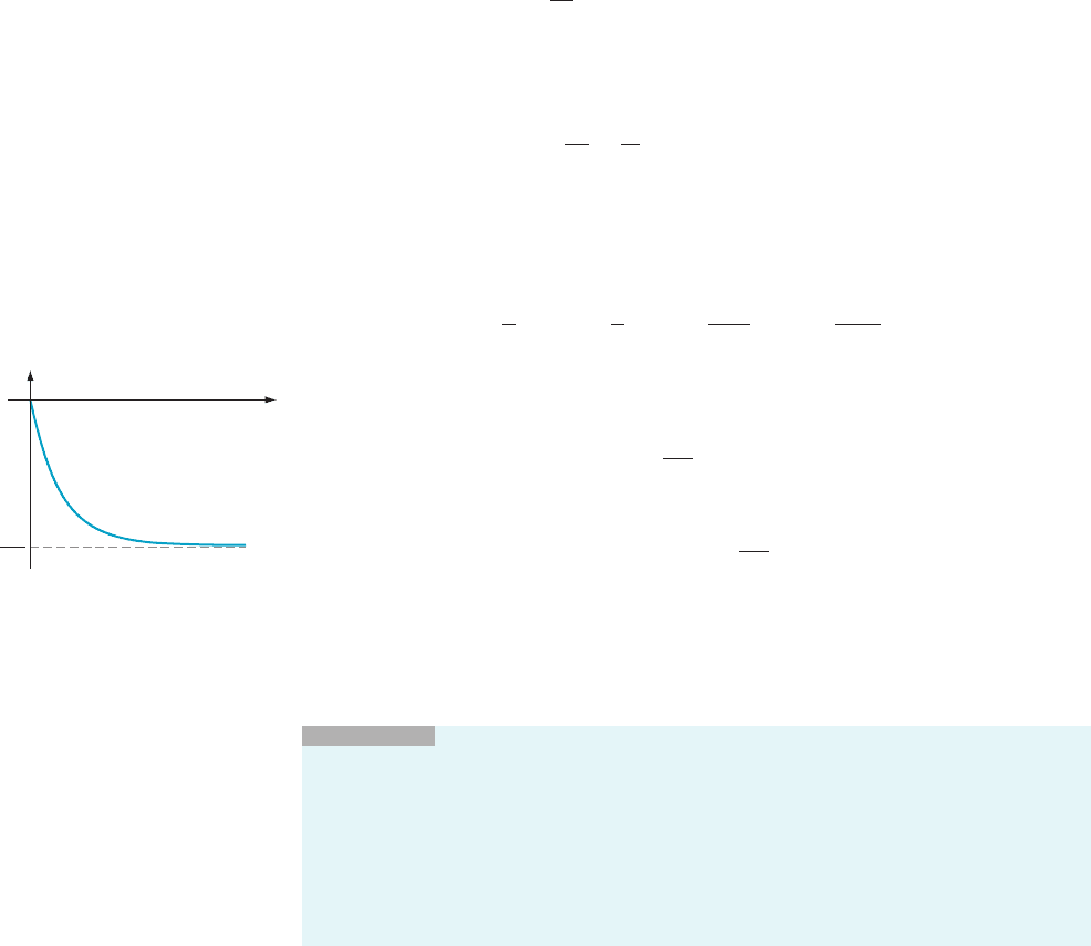
⁄ EX

AMPLE 7 Let v(t) denote the velocity at time t of an object of mass m

that is dropped from a great height. Assuming that air resistance is given by the

formula (7.7.12), determine v(t). What is the behavior of v(t) for large t?

Solution Denot

ing the acceleration due to gravity by the positive constant g,we

write the downward force of gravity as 2m g. The equation of motion is therefore

mass 3 acceleration

|ﬄﬄﬄﬄﬄﬄﬄﬄﬄﬄﬄ{zﬄﬄﬄﬄﬄﬄﬄﬄﬄﬄﬄ}

Total Force

52k  v

|ﬄﬄ{zﬄﬄ}

Resistive Force

1 ð2m  gÞ

|ﬄﬄﬄﬄﬄ{zﬄﬄﬄﬄﬄ}

Force of gravity

On dividing by m and bringing v to the left side, we obtain the initial value problem

 v 52g; vð0Þ5 0:

This initial value problem is of the form (7.7.6) with unknown function v instead of y.

To complete the correspondence, we set α 52g, β 5 k/m,andy

5 v(0) 5 0 in (7.7.6).

The solution to our initial value problem is then obtained by using these values for the

constants and replacing y with v in equation (7.7.7). We obtain

vðtÞ5





2βt

|ﬄﬄﬄﬄﬄﬄﬄﬄﬄﬄﬄﬄﬄﬄﬄ{zﬄﬄﬄﬄﬄﬄﬄﬄﬄﬄﬄﬄﬄﬄﬄ}

right side of ð7:7:7Þ

k=m



0 2

ð2gÞ

k=m



2kt=m

;

vðtÞ52



1 2 e

2kt=m



: ð7:7:13Þ

From this formula, we can calculate

lim

t-N

vðtÞ52

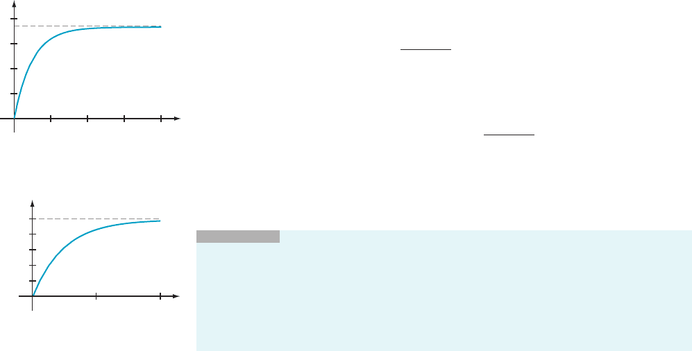
The quantity 2mg/k is said to be the terminal velocity of the falling object. This

terminology is somewhat misleading: Terminal velocity is approached arbitrarily

closely but is not attained. Figure 5 shows the graph of v and its horizontal

asymptote v 52mg /k.

INSIGHT

One of the reasons that students from so many different backgrounds

study calculus is its wide applicability. Mathematicians will often state a theorem in a

general form (such as the formulation of Theorem 2) in order to maximize the theorem’s

scope. We have already seen that the differential equation studied in Theorem 2 applies

to problems concerning heat transfer and motion. Here are four more applications of the

same differential equation.

1. A drug delivered intravenously to a patient enters his bloodstream at a constant

rate. The drug is broken down and eliminated from the patient’s body at a rate that

v(t)



m Figure 5 Plot of velocity dur-

ing a fall under gravity, assuming

the linear drag law

614 Chapter 7 Applications of the Integral