Coburn J.W., Herdlick J.D. College Algebra: Graphs and Models
Подождите немного. Документ загружается.

112. From Example 11, (a) what is the significance of
the y-intercept? (b) If the domain were extended to
include what happens when x is
approximately 12.8?
113A. It is often said that while the difference of two
squares is factorable,
the sum of two squares is prime. To be 100%
correct, we should say the sum of two squares
cannot be factored using real numbers. If
complex numbers are used,
. Use this idea to
factor the following binomials.
a. b.
c.
113B. It is often said that while is factorable as
a difference of squares,
is not. To be
100% correct, we should say that is not
factorable using integers. Since , it
can actually be factored in the same way:
. Use this idea
to solve the following equations.
a. b.
c.
114. Every general cubic equation
can be written in the form
(where the squared term has been
“depressed”), using the transformation
Use this transformation to solve the
following equations.
a.
b.
w
3
6w
2
21w 26 0
w
3
3w
2
6w 4 0
w x
b
3a
.
q 0
x
3
px cw d 0
aw
3
bw
2
x
2
18 0
x
2
12 0x
2
7 0
x
2
17 1x 11721x 1172
1117
2
2
17
x
2
17
a
2
b
2
1a b21a b2, x
2
17
x
2
16
r1x2 x
2
7
q1x2 x
2
9p1x2 x
2
25
1a
2
b
2
2 1a bi21a bi2
a
2
b
2
1a b21a b2,
0 6 x 13,
410 CHAPTER 4 Polynomial and Rational Functions 4–30
College Algebra G&M—
Note: It is actually very rare that the transformation
produces a value of for the “depressed”
cubic and general solutions must
be found using what has become known as
Cardano’s formula. For a complete treatment of
cubic equations and their solutions, visit our
website at www.mhhe.com/coburn.
115. For each of the following complex polynomials,
one of its zeroes is given. Use this zero to help
write the polynomial in completely factored form.
(Hint: Synthetic division and the quadratic formula
can be applied to all polynomials, even those with
complex coefficients.)
a.
b.
c.
d.
e.
f.
g.
h.
z 2 3i
C1z2 z
3
2z
2
119 6i2z 120 30i2;
z 2 i
C1z2 z
3
12 i2z
2
15 4i2z 16 3i2;
z 4i
z 44i;C1z2 z
3
16 4i2z
2
111 24i2
z 6i
C1z2 z
3
12 6i2z
2
14 12i2z 24i;
z i
C1z2 z
3
14 i2z
2
129 4i2z 29i;
z 3i
C1z2 z
3
12 3i2z
2
15 6i2z 15i;
z 9i
C1z2 z
3
15 9i2z
2
14 45i2z 36i;
z 4i
C1z2 z
3
11 4i2z
2
16 4i2z 24i;
x
3
px q 0,
q 0
䊳
MAINTAINING YOUR SKILLS
116. (2.5) Graph the piecewise-defined function and
find the values of f(2), and f(5).
117. (3.4) For a county fair, officials need to fence off a
large rectangular area, then subdivide it into three
equal (rectangular) areas. If the county provides
1200 ft of fencing, (a) what dimensions will
maximize the area of the larger (outer) rectangle?
(b) What is the area of each smaller rectangle?
f
1x2 •
2 x 1
冟
x 1
冟
1 6 x 6 5
4 x 5
f
132,
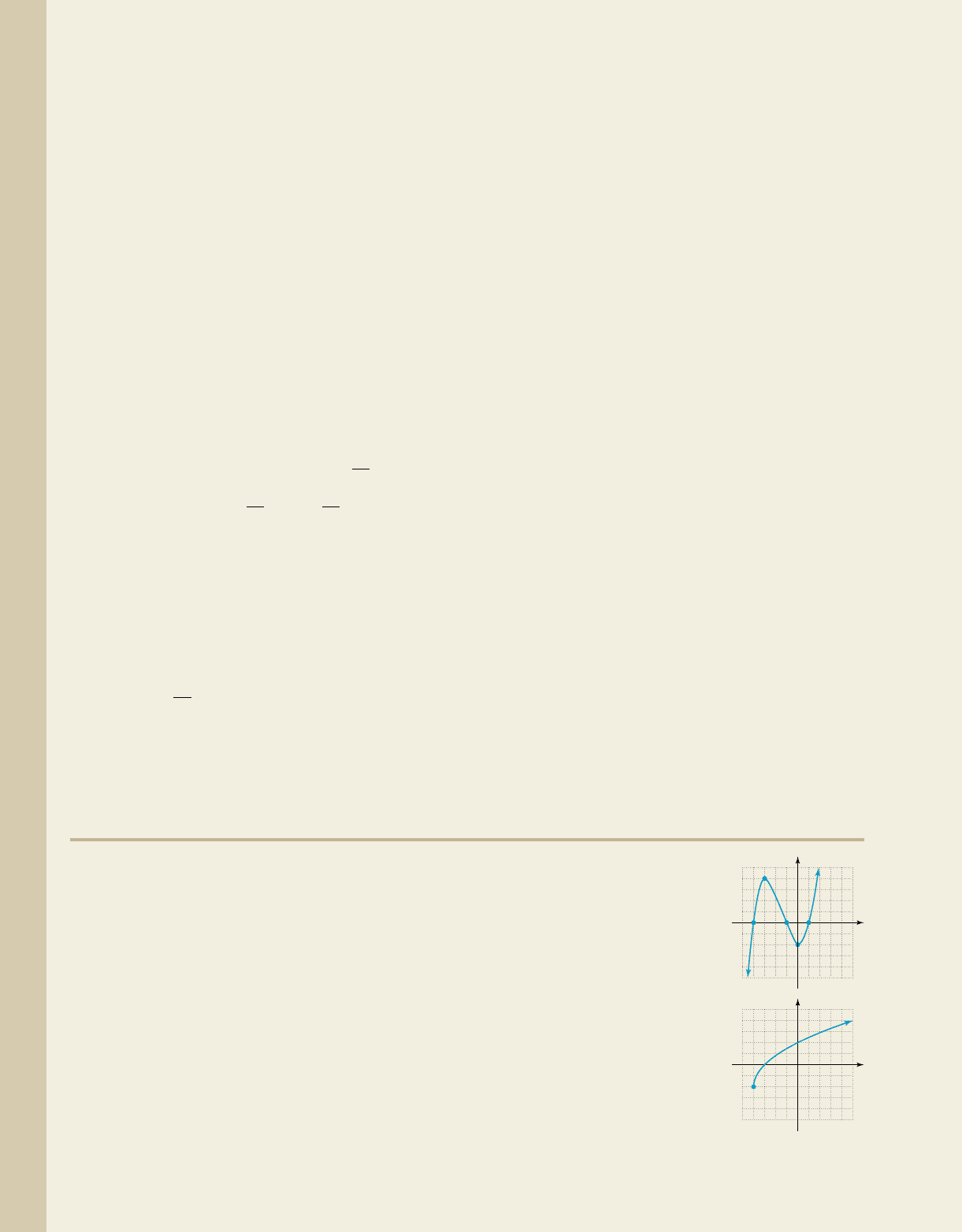
118. (2.1) Use the graph given
to (a) state intervals where
(b) locate local
maximum and minimum
values, and (c) state
intervals where
and
119. (2.2) Write the equation of the
function shown.
f
1x2T.
f
1x2c
f
1x2 0,
x
y
f(x)
5
5
5
5
x
y
55
5
5
r(x)
cob19545_ch04_381-410.qxd 8/19/10 10:36 PM Page 410
College Algebra Graphs & Models—
As with linear and quadratic functions, understanding graphs of polynomial functions
will help us apply them more effectively as mathematical models. Since all real poly-
nomials can be written in terms of their linear and quadratic factors (Section 4.2), these
functions provide the basis for our continuing study.
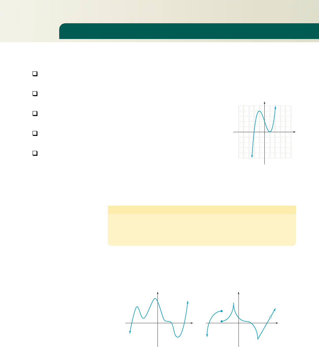
A. Identifying the Graph of a Polynomial Function
Consider the graphs of and
which we know are smooth, continuous
curves. The graph of f is a straight line with positive
slope, that crosses the x-axis at The graph of g is a
parabola, opening upward, shifted 1 unit to the right,
and touching the x-axis at When fand gare “com-
bined” into the single function
the behavior of the graph at these zeroes is still evident.
In Figure 4.9, the graph of P crosses the x-axis at
“bounces” off the x-axis at and is still
a smooth, continuous curve. This observation could
be extended to include additional linear or quadratic
factors, and helps affirm that the graph of a polyno-
mial function is a smooth, continuous curve.
Further, after the graph of P crosses the axis at it must “turn around” at some
point to reach the zero at then turn again as it touches the x-axis without crossing.
By combining this observation with our work in Section 4.2, we can state the following:
Polynomial Graphs and Turning Points
1. If P(x) is a polynomial function of degree n,
then the graph of P has at most turning points.
2. If the graph of a function P has turning points,
then the degree of P(x) is at least n.
While defined more precisely in a future course, we will take “smooth” to mean
the graph has no sharp turns or jagged edges, and “continuous” to mean the entire
graph can be drawn without lifting your pencil (Figure 4.10). In other words, a polyno-
mial graph has none of the attributes shown in Figure 4.11.
n 1
n 1
x 1,
x 2,
x 1,x 2,
P1x2 1x 221x 12
2
,
x 1.
2.
1x 12
2
,g1x2
f
1x2 x 2
LEARNING OBJECTIVES
In Section 4.3 you will see
how we can:
A. Identify the graph of a
polynomial function and
determine its degree
B. Describe the end-
behavior of a polynomial
graph
C. Discuss the attributes of
a polynomial graph with
zeroes of multiplicity
D. Graph polynomial
functions in standard
form
E. Solve applications of
polynomials and
polynomial modeling
5
5
54
4
43
3
2
1
5
4
3
2
1
113
x
y
2
2
P(x)
Figure 4.9
polynomial nonpolynomial
gap
cusp
hole
sharp turn
Figure 4.10 Figure 4.11
4–31 411
4.3 Graphing Polynomial Functions
cob19545_ch04_411-429.qxd 8/19/10 11:10 PM Page 411
412 CHAPTER 4 Polynomial and Rational Functions 4–32
College Algebra Graphs & Models—College Algebra Graphs & Models—
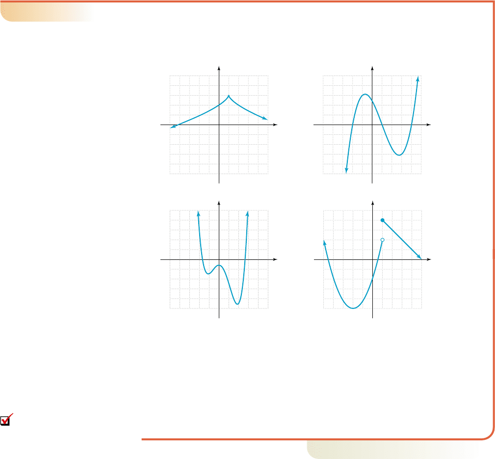
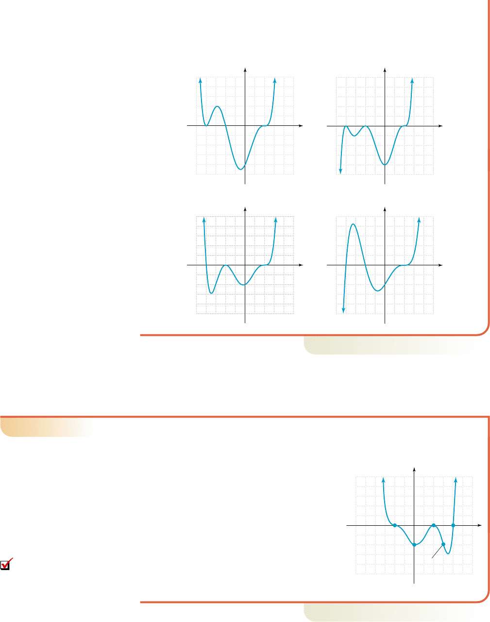
EXAMPLE 1
䊳
Identifying Polynomial Graphs
Determine whether each graph could be the graph of a polynomial. If not, discuss
why. If so, use the number of turning points and zeroes to identify the least
possible degree of the function.
a. b.
x
y
543215 4 3 2 1
5
4
3
2
1
5
4
3
2
1
x
y
543215 4 3 2 1
5
4
3
2
1
5
4
3
2
1
c. d.
Solution
䊳
a. This is not a polynomial graph, as it has a cusp at (1, 3).
A polynomial graph is always smooth.
b. This graph is smooth and continuous, and could be that of a polynomial.
With two turning points and three zeroes, the function is at least degree 3.
c. This graph is smooth and continuous, and could be that of a polynomial.
With three turning points and two zeroes, the function is at least degree 4.
d. This is not a polynomial graph, as it has a gap (discontinuity) at .
A polynomial graph is always continuous.
Now try Exercises 7 through 12
䊳
B. The End-Behavior of a Polynomial Graph
Once the graph of a function has “made its last turn” and crossed or touched its last real
zero, it will continue to increase or decrease without bound as becomes large. As
before, we refer to this as the end-behavior of the graph. In previous sections, we noted
that quadratic functions (degree 2) with a positive leading coefficient had the
end-behavior “up on the left” and “up on the right (up/up).” If the leading coefficient
was negative end-behavior was “down on the left” and “down on the right
(down/down).” These descriptions were also applied to the graph of a linear function
(degree 1). A positive leading coefficient indicates the graph will
be down on the left, up on the right (down/up), and so on. All polynomial graphs ex-
hibit some form of end-behavior, which can be likewise described.
1m 7 02y mx b
1a 6 02,
1a 7 02,
冟
x
冟
x 1
x
y
543215 4 3 2 1
5
4
3
2
1
5
4
3
2
1
x
y
543215 4 3 2 1
5
4
3
2
1
5
4
3
2
1
A. You’ve just seen how
we can identify the graph of a
polynomial function and
determine its degree
cob19545_ch04_411-429.qxd 8/19/10 11:10 PM Page 412
4–33 Section 4.3 Graphing Polynomial Functions 413
College Algebra Graphs & Models—
EXAMPLE 2
䊳
Identifying the End-Behavior of a Graph
State the end-behavior of each graph shown:
a. b. c. h1x22x
4
5x
2
x 1g1x22x
5
7x
3
4xf 1x2 x
3
4x 1
Solution
䊳
a. down on the left, up on the right b. up on the left, down on the right
c. down on the left, down on the right
Now try Exercises 13 through 16
䊳
The leading term of a polynomial function is said to be the dominant term,
because for large values of , the value of is much larger than all other terms com-
bined. Figure 4.12 shows a table of values for ,
where the leading coefficient is positive and very small, with all other coefficients
negative and much larger. Initially, all outputs are negative as these terms overpower
the leading term. But eventually (in this case for any integer greater than 10), the lead-
ing term will dominate all others since it becomes much more “powerful” for larger
values. See Figure 4.13.
This means that like linear and quadratic graphs, polynomial end-behavior can be
predicted in advance by analyzing this term alone.
1. For when n is even, any nonzero number raised to an even power is positive,
so the ends of the graph must point in the same direction. If both point up-
ward. If both point downward.
2. For when n is odd, any number raised to an odd power has the same sign as the
input value, so the ends of the graph must point in opposite directions. If
end-behavior is down on the left, up on the right. If end-behavior is up on
the left, down on the right.
From this we find that end-behavior depends on two things: the degree of the function
(even or odd) and the sign of the leading coefficient (positive or negative). In more formal
terms, this is described in terms of how the graph “behaves” for large values of x. For end-
behavior that is “up on the right,” we mean that as x becomes a large positive number, y
becomes a large positive number. This is indicated using the notation: as
Similar notation is used for the other possibilities. These facts are summarized in
Table 4.1. The interior portion of each graph is dashed since the actual number of turning
x Sq, y Sq.
a 6 0,
a 7 0,
ax
n
a 6 0,
a 7 0,
ax
n
Y
1
0.4x
5
3x
4
9x
3
15x
2
30
Figure 4.12
Figure 4.13
Y
1
0.4x
5
3x
4
9x
3
15x
2
30
ax
n
冟
x
冟
ax
n
x
y
543215 4 3 2 1
5
4
3
2
1
5
4
3
2
1
x
y
543215 4 3 2 1
5
4
3
2
1
5
4
3
2
1
x
y
543215 4 3 2 1
5
4
3
2
1
5
4
3
2
1
WORTHY OF NOTE
As a visual aid to end-behavior, it
might help to picture a signalman
using semaphore code as
illustrated here. As you view the
end-behavior of a polynomial
graph, there is a striking
resemblance.
up/up down/down
up/down down/up
cob19545_ch04_411-429.qxd 8/19/10 11:10 PM Page 413
Note the end-behavior of can be used as a representative of all odd degree func-
tions, and the end-behavior of as a representative of all even degree functions.
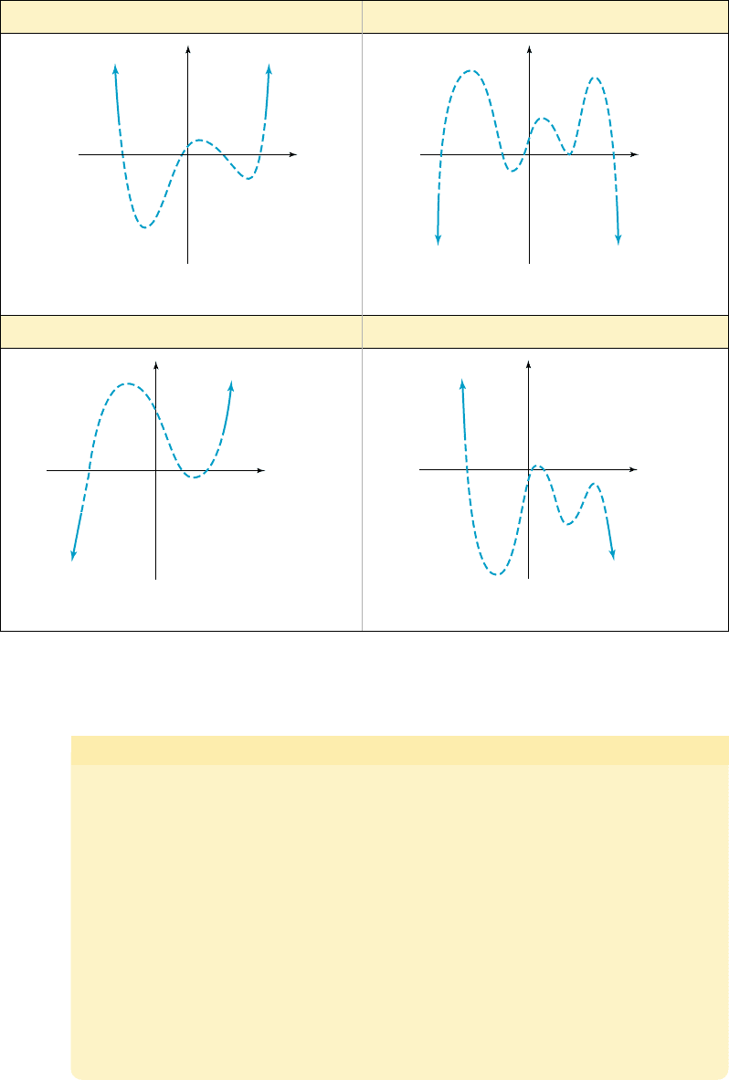
The End-Behavior of a Polynomial Graph
Given a polynomial P(x) with leading term and
If n is even, ends will point in the same direction,
1. for up on the left, up on the right (as with );
as as
2. for down on the left, down on the right (as with );
as as
If n is odd, the ends will point in opposite directions,
1. for down on the left, up on the right (as with );
as as
2. for up on the left, down on the right (as with );
as as x Sq, y S qx S q, y Sq;
y xa 6 0:
x Sq, y Sqx S q, y S q;
y xa 7 0:
x Sq, y S qx S q, y S q;
y x
2
a 6 0:
x Sq, y Sqx S q, y Sq;
y x
2
a 7 0:
n 1.ax
n
y ax
2
y mx
414 CHAPTER 4 Polynomial and Rational Functions 4–34
College Algebra Graphs & Models—
x
y
as x →
q, y → q as x → q, y →
q
up on the left, up on the right
(similar to y x
2
)
x
y
down on the left, down on the right
as x → q, y →
qas x →
q, y →
q
(similar to y x
2
)
x
y
as x → q, y → q
as x →
q, y →
q
down on the left, up on the right
(similar to y x)
Even Degree: a ⬎ 0 a ⬍ 0
Odd Degree: a ⬎ 0 a ⬍ 0
x
y
as x →
q, y → q
as x → q, y →
q
up on the left, down on the right
(similar to y x)
Table 4.1
Polynomial End-Behavior
points may vary, although a polynomial of odd degree will have an even number of turn-
ing points, and a polynomial of even degree will have an odd number of turning points.
cob19545_ch04_411-429.qxd 8/19/10 11:10 PM Page 414
4–35 Section 4.3 Graphing Polynomial Functions 415
College Algebra Graphs & Models—
EXAMPLE 3
䊳
Identifying the End-Behavior of a Function
State the end-behavior of each function.
a. b.
Solution
䊳
a. The function has degree 4 (even), so the ends will point in the same direction.
The leading coefficient is positive, so end-behavior is up/up. See Figure 4.14.
b. The function has degree 5 (odd), so the ends will point in opposite directions.
The leading coefficient is negative, so the end-behavior is up/down. See
Figure 4.15.
Now try Exercises 17 through 22
䊳
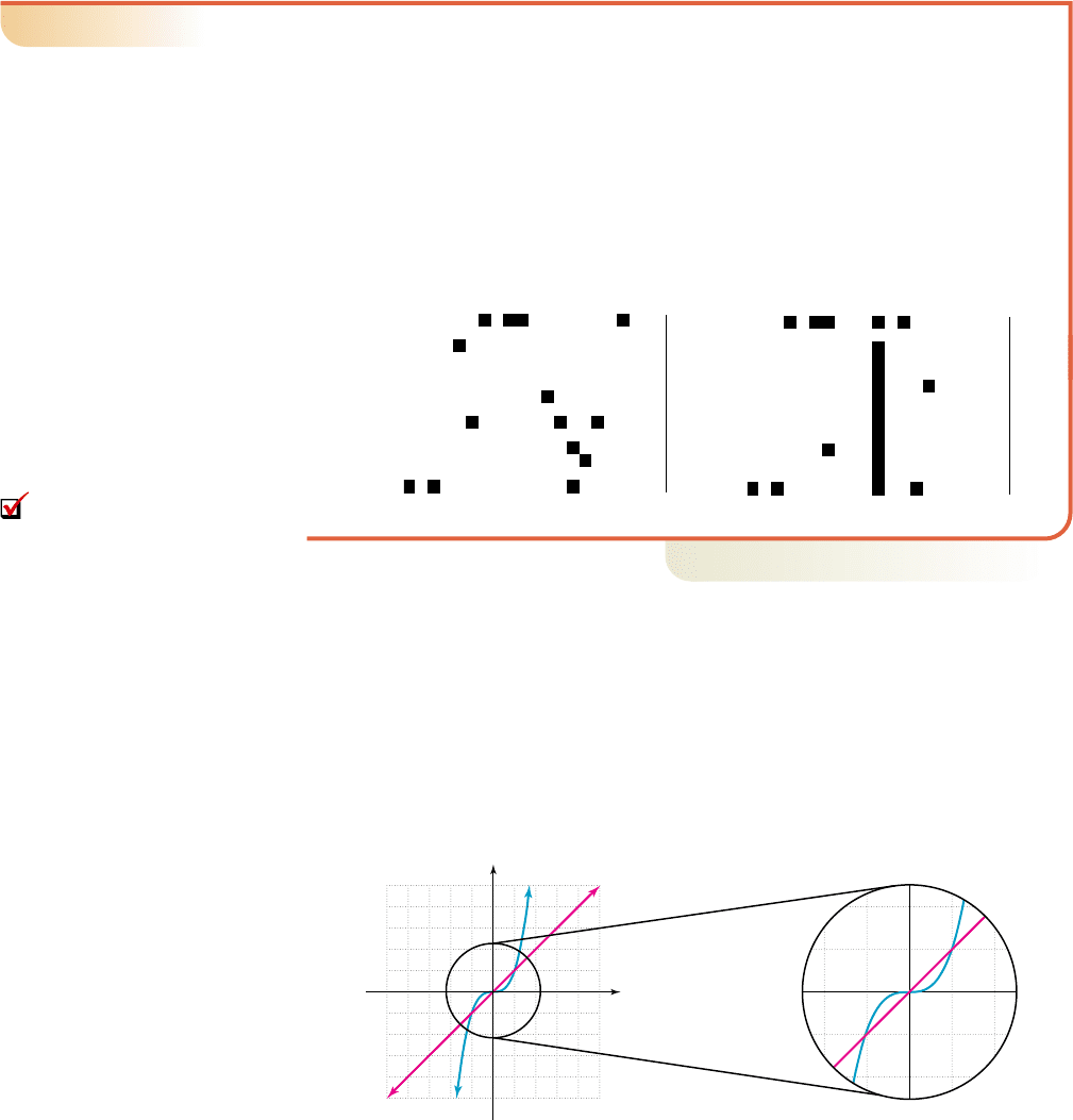
C. Attributes of Polynomial Graphs with Zeroes of Multiplicity
Another important aspect of polynomial functions is the behavior of a graph near its
zeroes. In the simplest case, consider the functions and in Fig-
ure 4.16. Both have odd degree, like end-behavior (down/up), and a zero at
But the zero of f has multiplicity 1, while the zero from g has multiplicity 3. Notice
the graph of g is vertically compressed near and flattens out on its approach
and departure from this zero.
This behavior can be explained by noting that for and 1, But for
the graph of g will be closer to the x-axis (g decreases faster than f ) since the
cube of a fractional number is smaller than the fraction itself. We further note that for
g increases much faster than f, and Similar observations can
be made regarding and in Figure 4.17. Both functions have even
degree, a zero at and for and 1. But for the func-
tion with higher degree is once again closer to the x-axis.
冟
x
冟
6 1,x 1f
1x2 g1x2x 0,
g1x2 x
4
f 1x2 x
2
0g1x207 0f 1x20.
冟
x
冟
7 1,
冟
x
冟
6 1,
f
1x2 g1x2.x 1
Figure 4.16
55
5
5
x
y
122 1
1
1
2
2
g(x) x
3
f(x) x
x 0
x 0.
g1x2 x
3
f 1x2 x
5
5
5
3
10
10
4
4
Figure 4.14 Figure 4.15
g1x22x
5
6x
3
1f 1x2 0.8x
4
3x
3
0.5x
2
4x 1
B. You’ve just seen how
we can describe the end-
behavior of a polynomial graph
cob19545_ch04_411-429.qxd 8/19/10 11:10 PM Page 415
These observations can be generalized and applied to all real zeroes of a function.
Polynomial Graphs and Zeroes of Multiplicity
Given P(x) is a polynomial with factors of the form with c a real number,
•Ifm is odd, the graph will cross through the x-axis.
•Ifm is even, the graph will “bounce” off the x-axis (touching at just one point).
In each case, the graph will be more compressed (flatter) near c for larger values of m.
To illustrate, compare the graph of (Figure 4.18), with the
graph of shown in Figure 4.19, noting the increased multi-
plicity of each zero.
Both graphs show the expected zeroes at and but the graph of p(x)
is flatter near and due to the increased multiplicity of each zero. We
also lose sight of the graph of p(x) between and since the increased
multiplicities produce larger values than the original grid could display.
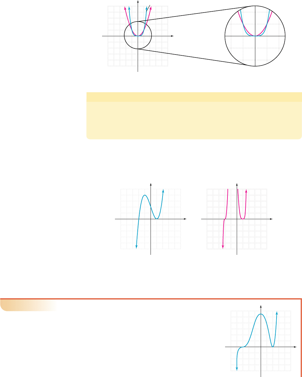
EXAMPLE 4
䊳
Naming Attributes of a Function from Its Graph
The graph of a polynomial is shown.
a. State whether the degree of f is even or odd.
b. Use the graph to name the zeroes of f, then
state whether their multiplicity is even or odd.
c. State the minimum possible degree of f.
d. State the domain and range of f.
f
1x2
x 0,x 2
x 1,x 2
x 1,x 2
x
y
543215 4 3 2 1
5
4
3
2
1
5
4
3
2
1
P(x)
x
y
543215 4 3 2 1
5
4
3
2
1
5
4
3
2
1
p(x)
Figure 4.18 Figure 4.19
p1x2 1x 22
3
1x 12
4
P1x2 1x 221x 12
2
1x c2
m
,
Figure 4.17
55
5
5
x
y
122 1
1
1
2
2
g(x) x
4
f(x) x
2
416 CHAPTER 4 Polynomial and Rational Functions 4–36
College Algebra Graphs & Models—
543215 4 3 2 1
4
6
8
2
12
8
6
4
2
x
y
10
f(x)
cob19545_ch04_411-429.qxd 8/19/10 11:11 PM Page 416
4–37 Section 4.3 Graphing Polynomial Functions 417
College Algebra Graphs & Models—
Solution
䊳
a. Since the ends of the graph point in opposite directions, the degree of the
function must be odd.
b. The graph crosses the x-axis at and is compressed near meaning it
must have odd multiplicity with The graph “bounces” off the x-axis at
and 2 must be a zero of even multiplicity.
c. The minimum possible degree of f is 5, as in
d. .
Now try Exercises 23 through 28
䊳
To find the degree of a polynomial from its factored form, add the exponents on all lin-
ear factors, then add 2 for each irreducible quadratic factor (the degree of any quadratic
factor is 2). The sum gives the degree of the polynomial, from which end-behavior can
be determined. To find the y-intercept, substitute 0 for x as before, noting this is equiv-
alent to applying the exponent to the constant from each factor.
EXAMPLE 5
䊳
Naming Attributes of a Function from Its Factored Form
State the degree of each function, then describe the end-behavior and name the
y-intercept of each graph.
a. b.
Solution
䊳
a. The degree of f is With even degree and positive leading
coefficient, end-behavior is up/up. For the y-intercept
is See Figure 4.20.
b. The degree of g is With odd degree and negative leading
coefficient, end-behavior is up/down. For the
y-intercept is (0, 100). See Figure 4.21.
Now try Exercises 29 through 36
䊳
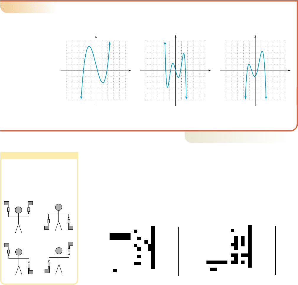
EXAMPLE 6
䊳
Matching Graphs to Functions Using Zeroes of Multiplicity
The following functions all have zeroes at and 1. Match each function
to the corresponding graph using its degree and the multiplicity of each zero.
a. b.
c. d.
Solution
䊳
The functions in Figures 4.22 and 4.24 must have even degree due to end-behavior,
so each corresponds to (a) or (d). At the graph in Figure 4.22 “crosses,”
while the graph in Figure 4.24 “bounces.” This indicates Figure 4.22 matches
equation (d), while Figure 4.24 matches equation (a).
x 1
y 1x 22
2
1x 121x 12
3
y 1x 22
2
1x 12
2
1x 12
3
y 1x 221x 121x 12
3
y 1x 221x 12
2
1x 12
3
x 2, 1,
100
100
5
5
200
1000
7
5
Figure 4.20 Figure 4.21
g1021122
2
152152 100,
2 2 1 5.
10, 242.
f
102 122
3
13224,
3 1 4.
g1x21x 22
2
1x
2
521x 52f 1x2 1x 22
3
1x 32
x 僆 ⺢, y 僆 ⺢
f 1x2 a1x 22
2
1x 32
3
.
x 2
m 7 1.
3,x 3
cob19545_ch04_411-429.qxd 8/19/10 11:11 PM Page 417
The graphs in Figures 4.23 and 4.25 must have odd degree due to end-behavior, so
each corresponds to (b) or (c). Here, one graph “bounces” at while the other
“crosses.” The graph in Figure 4.23 matches equation (c), the graph in Figure 4.25
matches equation (b).
Now try Exercises 37 through 42
䊳
Using the ideas from Examples 5 and 6, we’re able to draw a fairly accurate graph
given the factored form of a polynomial. Convenient values between two zeroes, called
midinterval points, should be used to help complete the graph.
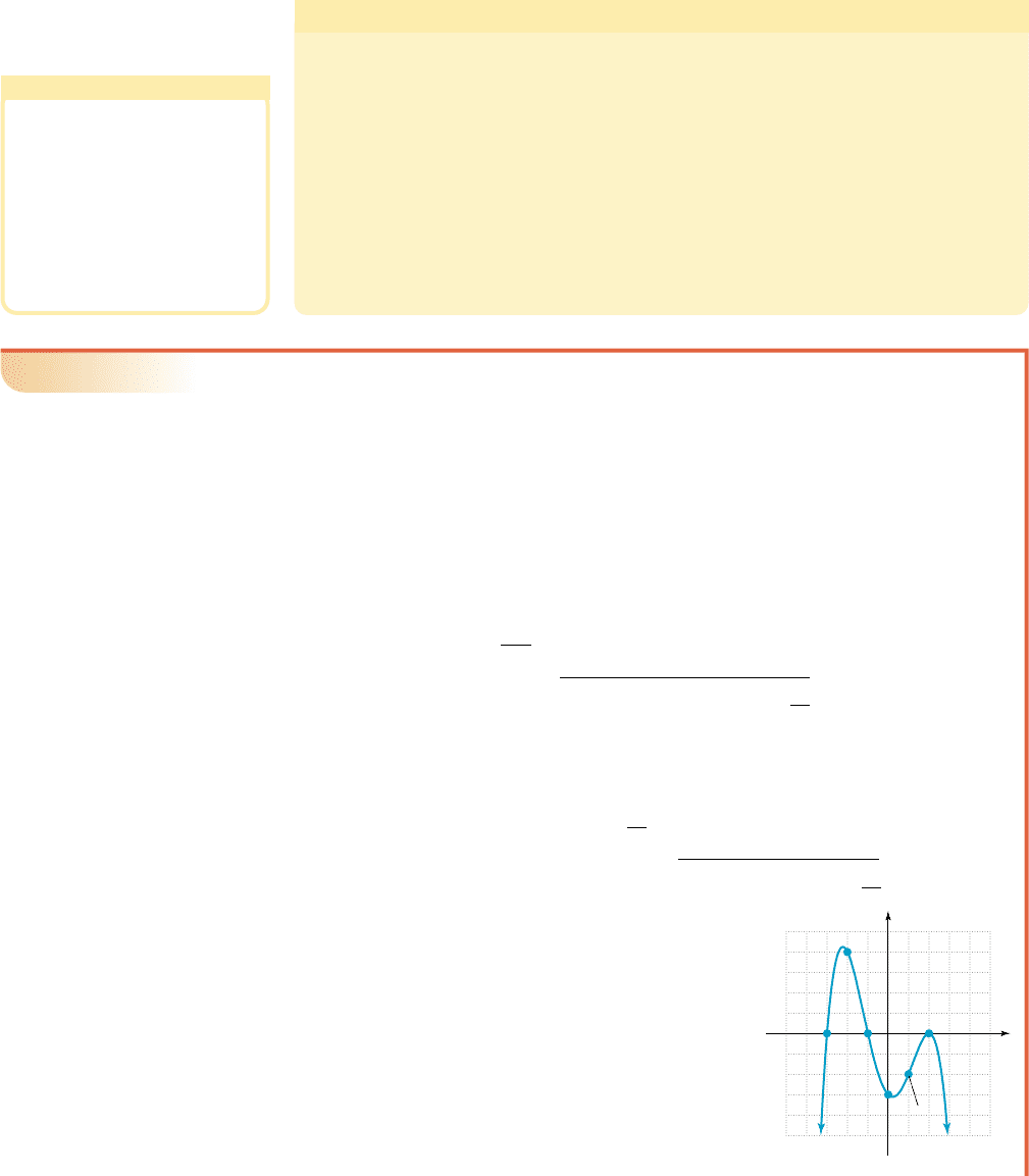
EXAMPLE 7
䊳
Graphing a Function Given the Factored Form
Sketch the graph of using end-behavior; the
x- and y-intercepts, and zeroes of multiplicity.
Solution
䊳
Adding the exponents of each factor, we find
that f is a function of degree 6 with a positive
lead coefficient, so end-behavior will be up/up.
Since the y-intercept is The
graph will bounce off the x-axis at (even
multiplicity), and cross the axis at and 2
(odd multiplicities). The graph will “flatten out”
near because of its higher multiplicity.
To help “round-out” the graph we evaluate f at
giving
(note scaling of the x- and y-axes).
Now try Exercises 43 through 56
䊳
10.5210.52
2
12.52
3
⬇ 1.95x 1.5,
x 1
x 1
x 1
10, 22.f
1022,
f
1x2 1x 221x 12
2
1x 12
3
x 2,
418 CHAPTER 4 Polynomial and Rational Functions 4–38
College Algebra Graphs & Models—
212 1
5
4
3
2
1
5
4
3
2
1
x
y
2112
5
4
3
2
1
5
4
3
2
1
x
y
Figure 4.22 Figure 4.23
212 1
5
4
3
2
1
5
4
3
2
1
x
y
212 1
5
4
3
2
1
5
4
3
2
1
x
y
Figure 4.24 Figure 4.25
3213 2 1
5
5
x
y
(1, 0) (2, 0)
(1, 0)
(0, 2)
(1.5, 1.95)
C. You’ve just seen how
we can discuss the attributes
of a polynomial graph with
zeroes of multiplicity
cob19545_ch04_411-429.qxd 8/19/10 11:11 PM Page 418
4–39 Section 4.3 Graphing Polynomial Functions 419
College Algebra Graphs & Models—
D. The Graph of a Polynomial Function
Using the cumulative observations from this and previous sections, a general strategy
emerges for the graphing of polynomial functions.
Guidelines for Graphing Polynomial Functions
1. Determine the end-behavior of the graph.
2. Find the y-intercept
3. Find the zeroes using any combination of the rational zeroes theorem, the
factor and remainder theorems, tests for 1 and , factoring, and
the quadratic formula.
4. Use the y-intercept, end-behavior, the multiplicity of each zero, and
midinterval points as needed to sketch a smooth, continuous curve.
Additional tools include (a) polynomial zeroes theorem, (b) complex conjugates
theorem, (c) number of turning points, (d) Descartes’ rule of signs, (e) upper and
lower bounds, and (f) symmetry.
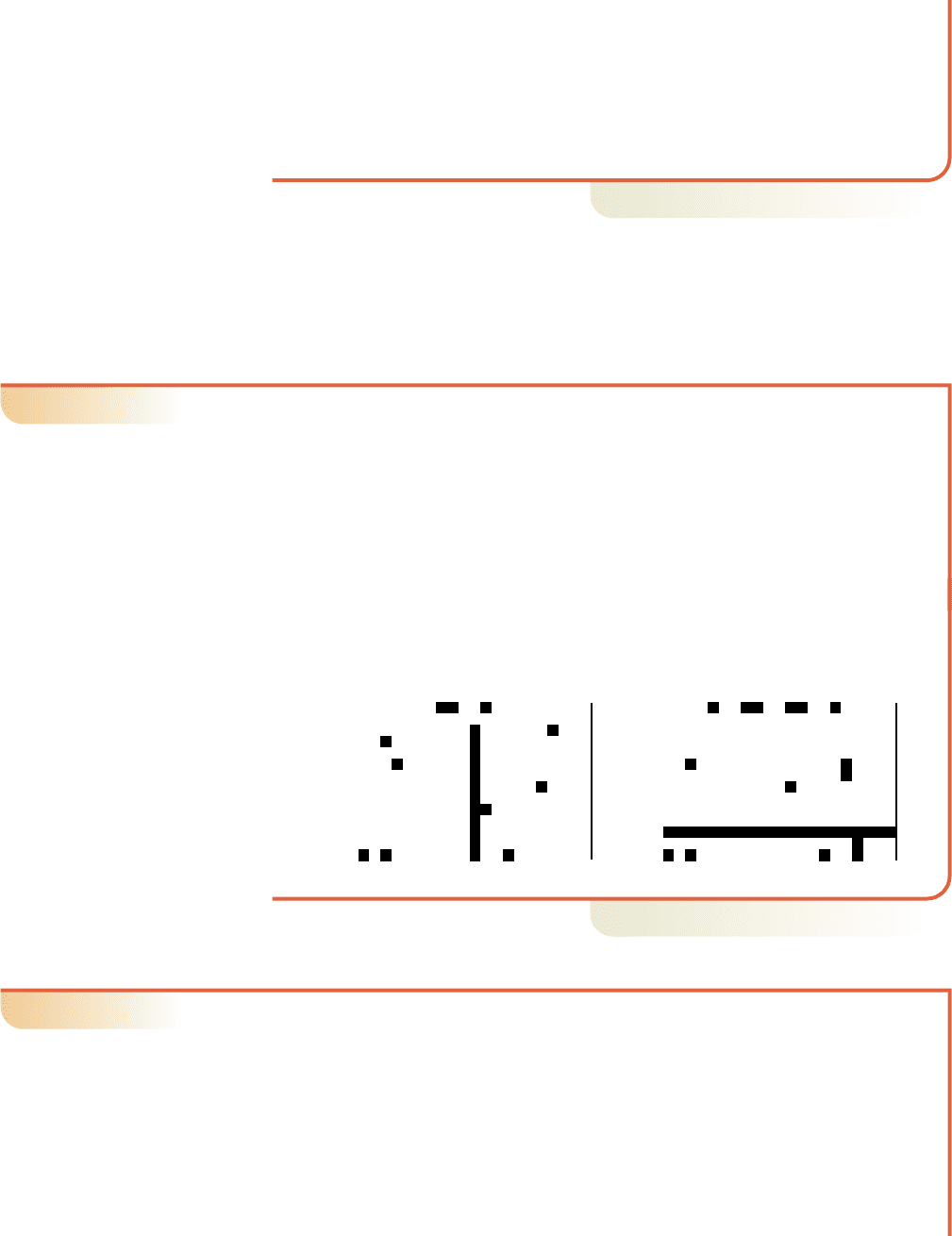
EXAMPLE 8
䊳
Graphing a Polynomial Function
Sketch the graph of
Solution
䊳
1. End-behavior: The function has degree 4 (even) with a negative leading
coefficient, so end-behavior is down on the left, down on the right.
2. Since the y-intercept is
3. Zeroes: Using the test for gives showing
is not a zero but is a point on the graph. Using the test for
gives so is a zero and is a factor.
Using with the factor theorem yields
The quotient polynomial is not easily factorable so we continue with synthetic
division. Using the rational zeroes theorem, the possible rational zeroes are
so we try
This shows is a zero, is a factor,
and the function can now be written as
Factoring from the trinomial gives
The zeroes of g are and both with
multiplicity 1, and with multiplicity 2.x 2
3,x 1
11x 121x 22
2
1x 32
11x 121x 221x 321x 22
g1x2 11x 121x 221x
2
x 62
1
g1x2 1x 121x 221x
2
x 62.
x 2x 2
2
|
11812
2 212
1 16
|
0
x 2.51, 12, 2, 6, 3, 46,
1
|
10 9 4 12
1 1 812
11 812
|
0
x 1
1x 1211 9 4 12 0,x 1
11, 82x 1
1 9 4 12 8,x 1
10, 122.g10212,
g1x2x
4
9x
2
4x 12.
1
10, a
0
2
WORTHY OF NOTE
Although of somewhat limited value,
symmetry (item f in the guidelines)
can sometimes aid in the graphing
of polynomial functions. If all terms
of the function have even degree,
the graph will be symmetric to the
y-axis (even). If all terms have odd
degree, the graph will be symmetric
to the origin. Recall that a constant
term has degree zero, an even
number.
use 2 as a “divisor” on
the quotient polynomial
55
20
20
Down on
left
Down on
right
(3, 0)
(2, 16)
(1, 0)
(0, 12)
(1, 8)
(2, 0)
g(x)
x
y
cob19545_ch04_411-429.qxd 8/19/10 11:11 PM Page 419