Edelstein-Keshet L. Mathematical Models in Biology
Подождите немного. Документ загружается.

386
Spatially
Distributed Systems
and
Partial
Differential
Equation
Models
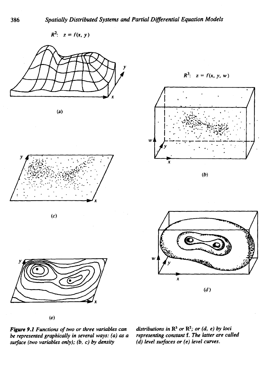
Figure
9.1
Functions
of
two or
three variables
can
be
represented graphically
in
several ways:
(a) as a
surface
(two
variables only);
(b, c) by
density
iistributions
in R
3
or R
2
; or (d, e) by
loci
^presenting constant
f. The
latter
are
called
'd)
level
surfaces
or (e)
level
curves.
Such loci
are a
generalized version
of
level curves,
but for
obvious reasons these
are
called
level
surfaces
[see Figure 9.l(d)].
To
clarify
with
an
example, consider
a
temperature
field in
three dimensions.
The
equitherms
are
then surfaces
at
which
some given constant temperature
is
maintained.
If
heat sources
are
located
at two
points,
the
resulting equithermal surfaces might look something like those shown
in
Figure
9.
l(d).
In
the
context
of
this chapter, level curves
or
surfaces might represent
the
loci
on
which
(1)
population density
is
constant
or (2)
chemical concentration
is
con-
stant.
We
shall
be
concerned primarily with statements about
how
spatial distribu-
tions change with time; frequently
it
will
be
clear that
the
movement
of one
sub-
stance
or
population
is
closely linked
to the
distribution
of
another.
Consider
the
following simple example.
An
organism crawling
on a flat
sur-
face
may
adapt
its
motion
to the
search
for
food particles. Imagine then that
the
dots
in
Figure
9.1(c)
represent nutrient particle concentration.
The
observed path should
ideally lead
to the
site
of
greatest concentration.
To
sense
an
increase
in the
ambient
concentration
level,
an
organism must continually
cross
level curves
of the
particle
distribution.
Per
unit distance traveled, this crossing
can be
done most efficiently
by
maintaining
a
path
orthogonal
to the
level curves;
in
other words,
a
tangent vector
to
the
path should
be
perpendicular
to a
tangent
to a
level curve through
a
given point.
This assertion
can be
verified using rather elementary calculus
of
several variables.
It can
also
be
shown that
the
destination will
be a
critical
point
of the
function
(in
this case
a
local
maximum)
but not
necessarily
the
global
maximum.
In
calculus
a
commonplace analogy
is
often
drawn
in
explaining these ideas.
Hikers
often
use
topographical maps which
are
two-dimensional representations
of
the
height
of the
terrain.
The
curves
on
such maps
are
level curves
for the
function
f(x,
y) =
height above
sea
level
at
latitude
x and
longitude
y.
Mountain peaks, val-
leys,
and
mountain passes
are
critical points
of
f(x,
y)
that correspond
to
local max-
ima,
minima,
and
saddle points respectively. Using local information only (for
ex-
ample, walking uphill with
no
information other than
the
local slope),
one can
attain
a
local maximum,
but
this
may or may not be the
highest possible peak.
These two-dimensional examples
can be
extended
to
higher dimensions.
A
motile organism that swims
in a
droplet
of
water might also
use
local cues
in
orient-
ing
itself
and
moving towards sites
mat
have higher nutrient levels. This type
of mo-
tion, called chemotaxis, will
be
discussed
at
greater length
in
Section 10.2.
In R
3
the
path
of a
highly
efficient
chemotactic organism would
be
orthogonal
to the
level sur-
faces
of the
nutrient distribution c(x,
y, z).
The
descriptive statements
in
this section
can be
made more
rigorous by
intro-
ducing
partial derivatives
and
gradients which
are
reviewed
in the
boxed material.
Several examples follow
the
general discussion
and
definitions.
Partial
Differential
Equations
and
Diffusion
in
Biological
Settings
387
In
/?
3
the
function
of
three variables given
by (2) can
similarly
be
represented
by
sets
of
points
for
which
388
Spatially
Distributed
Systems
and
Partial
Differential
Equation
Models
Note:
Equation (6c)
also
defines
the
equivalent notation used
for
multiple partial
differ-
entiation.
Partial
Derivatives
(A
Review)
For a
function
of two
variables/(x,
v) we
define
A
similar definition holds
for
df/dy.
Shorthand notation
for
partial derivatives
is
f
x
and/,.
To
understand
the
geometrical meaning
of
these derivatives, imagine standing
at
a
point
Cc
0
,
yo) on a
plane.
Suppose
/(x
0
,
y<>)
is the
height
of a
surface above this loca-
tion.
The
expression following "lim"
in
equation
(5)
(and similarly
for
df/dy)
repre-
sents
the
changes
in the
height
of the
surface
per
unit distance
as we
take
a
step
in the x
(or the y)
direction.
A
partial derivative
is the
limit
of
this quantity
as the
length
of the
step
shrinks
to an
infinitesimal
size.
It is
therefore analogous
to an
ordinary derivative
and
also represents
a
slope.
To
clarify, suppose
we
slice
away part
of the
surface
z =
f(x,
y)
along
a
direc-
tion parallel
to the x (or v)
axis. (See Figure 9.2.)
In
such cutaway drawings
the
partial
derivative
is the
slope
of a
tangent
to the
curve forming
the
surface edge.
The
idea
of a
partial derivative
is a
special case
of the
somewhat more general concept
of
directional
derivative.
We
shall
not
deal
in
more depth with this
but
rather refer
the
reader
to any
standard calculus text
for a
definition
and
explanation.
The
following properties
of
partial derivatives
follow
from
their basic definition:
for
functions
/ and g and
constan Similar equations ensue
for
partial differentiation
with
respect
to v.
For
functions that
are
c ously differentiable
sufficiently
many
times, it is
also true that mixed partial differentiation
in any
order produces
the
same result.
For
example
Partial
Differential
Equations
and
Diffusion
in
Biological
Settings
389
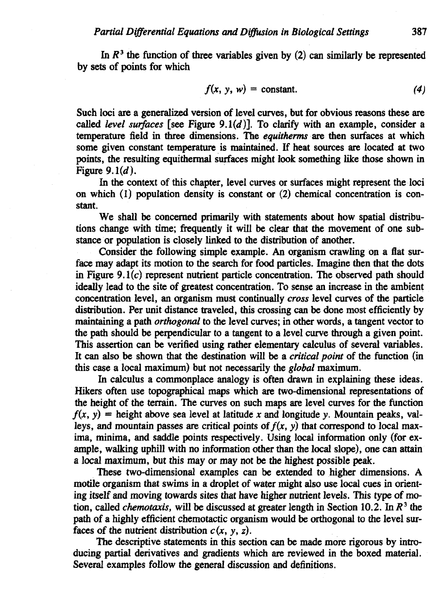
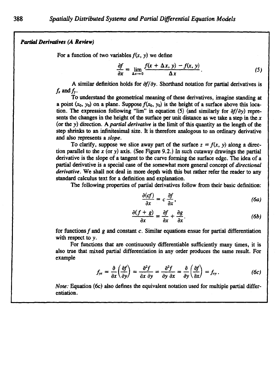
Figure
9.2 An
interpretation
of
partial
derivatives
and
gradient vectors.
The
surface
z
=
f(x,
y)
intersects
planes
for
which
y =
constant
or x =
constant along curves
€i and
€2.
The
slope
of
a
tangent
to i\ is
df/B\,
and
the
slope
of
a
tangent
to €
2
is
df/dy.
Gradient
vectors,
Vf
[for
f =
f(x,
y)]
live
in
the
xy
plane
and
have
(df/dx,
df/dy)
as
components.
These vectors
are
always
orthogonal
to
level curves
ofz —
f(x,
y),
shown
here
by
dashed lines (see inset).
Gradients
For a
function/of
several
variables
the
gradient,
symbolized
V/, is a
vector consisting
of
the
partial
derivatives
of/.
For
example,
iff
=
/(x,
y),
then
and so on for
functions
of n
variables.
The
symbol
V is
called
the del
operator,
and is
discussed
in
greater
detail
in
Section
9.3.
The
gradient
vector
has the
following
properties:
1. The
magnitude
of V/,
\Vf\,
represents
the
steepness
of the
local
variations
in the
•fimrtmn
f Prw
fvamnlp.
390
Spatially
Distributed
Systems
and
Partial
Differential
Equation Models
2. (a) The
direction
of
Vf,
is a
unit vector
in ine
direction
01
steepest {increasing; slope,
m tne
sense
that
a
step
in
this directi leads
to the
greatest increase
in/per
unit
distance,
(b) The
gradient vector
at
point Ot
0
,
yo) is
perpendicular
to a
level curve
f(x,
y) - c
that goes through
(XQ,
y
0
) as
long
as
(x
0
,
y
0
) is not a
local maxi-
mum,
minimum,
or
saddle point.
For
every point
in R
2
(analogously,
R
3
or
/?")
at
which
the
function/is
defined,
is
continuous,
and has
partial derivatives, there will
be a
gradient vector.
The
vector
will have
all
zero components
at the
critical points of/.
It is
common
to
visualize
a
whole collection
of
these vectors,
one at
each point
in
space,
as a
vector
field. A
vector
field
that
arises thus
is
called
a
gradient
field and has
certain
special
properties.
(Note that
a
gradient
field is a
vector
field, but the
converse
is not
necessarily true.)
Gradient
fields can
always
be
paired
(up to an
arbitrary constant)
with
differen-
tiable multivariate
functions
and
vice versa (see examples
in the
following
boxes).
We
see
that
the
variations
in a
spatial distribution lead
to
orientation cues that
are
repre-
sented
by the
geometry
of the
gradient
field.
The
proof
of the
statements
in
this
box are
based
on the
chain rule
of
functions
of
several
variables
and on the
properties
of
curves
and
vector
dot
products. These
can be
found
in any
text dealing
with
the
calculus
of
several variables.
Example
1
Consider
the
function
Level curves
of
this
function
have
the
equation
These
are
circles
of
radius c
1/2
centered
at the
point
(1,
-2). Partial derivatives
of
f(x,
y) are the
following:
Partial
Differential
Equations
and
Diffusion
in
Biological Settings
391
The
gradient
vector
at a
point
(x, y) is
This vector
is
perpendicular
to a
level curve going through
the
point
(x, y). A
critical point
of/occurs
at (1,
-2), where
Vf
= (0, 0). At
this
point,/(l,
-2) = 0. At
any
other
point/is
greater.
For
example,/(I,
1)
=1-2+1+4
+ 5 = 9.
There-
fore
(1,
—2)
is a
local minimum.
(A
more
rigorous
second-derivative
test
to
distinguish
between local minima, maxima,
and
saddle points
is
given
in
most calculus books).
Example
2
Consider
the
vector
field
We
would like
to
determine whether
F is a
gradient
field,
that
is,
whether there
is a
function/(AT,
y)
such that
If
so,
then
where M(x,
y) =
df/dx
and N =
df/dy.
By
a
previous observation
we
must
have
Checking this,
we
note that
so
that
no
contradiction
results by
assuming that (lla) holds.
The
condition given
by
(12)
in
fact
guarantees that
F is a
gradient
field (a
fact
whose proof
will
be
omitted
here).
To find/we
need
a
function whose partial derivatives satisfy
the
following:
392
Spatially Distributed Systems
and
Partial
Differential
Equation Models
Integrating each expression with respect
to a
single variable while holding
the
other
variable constant leads
to
these results:
and
In
ordinary one-variable calculus,
a
single integration introduces
a
single arbitrary con-
stant. However,
in the
partial integration
of
(14)
and
(15)
one
must account
for the
dis-
tinct possibility that
the
integration
"constants"
H and G may
depend
on the
values
given
to the fixed
variables
(to y =
const
and to x =
const).
For
this reason
it is
neces-
sary
to
presuppose that
are
functions.
Indeed,
the
only possibility
for
matching
the two
different
expressions,
(14)
and
(15), both
of
which equal
the
same function/(jc,
v),
would
be to
take
for
constant
c.
The
conclusion
then
is
that
To
check this result, observe that
which
confirms
the
calculation. Note that adding
any
constant
to
f(x,
y)
results
in
th<
same gradient.
Thus/(x,
v) is
defined
only
up to
some arbitrary additive constant.
Example
3
The
concentration
of
nutrient particles suspended
in a
pond
is
given
by the
expression
An
organism located
at (x, y, z) = (1,
—
1, 1)
moves
in the
direction
of
increasing
con
centration.
In
which direction should
it
move? Where
is the
maximum concentration?
Answer
To find the
direction
of
greatest increase
per
unit distance, compute
the
gradient vectoi
Since
c is a
function
of
three variables,
Vc is a
vector
in R
3
:
In
the
next section
our
purpose
is to
understand
the
basic process through which
a
partial differential description
of
motion through space
is
obtained.
We
shall
be
con-
cerned mainly with
the
dynamic
processes
that lead
to
changes
in a
spatial distribu-
tion over time. Some
of the
many examples cited pertain
to the
motion
and
continu-
ous
redistribution
of
animals,
cells,
and
molecules through space.
For
this reason
we
shall deal with functions that depend
on
both space
and
time.
9.2 A
QUICK DERIVATION
OF THE
CONSERVATION EQUATION
The
conservation equation
in its
various forms
is the
most fundamental statement
through
which changes
in
spatial distributions
are
described. Most
of the
PDEs
we
will
encounter
are
ultimately based
on
such
statements
of
balance.
To
gain
an
easy
familiarity
with
the
basic concepts
we
will consider
a
rather special case
and
give
an
informal
derivation
first,
later
to be
made more
rigorous and
more general.
Our
initial assumptions
are
that
1.
Motion takes place
in a
single space dimension (as,
for
example,
in the
thin
tube
of
Figure 9.3a).
2. The
cross-sectional area
of the
vessel
or
container
is
constant along
its
entire
length.
We
shall
let x
represent
the
distance
along
the
tube
from
some arbitrary
loca-
tion. Fixing attention
on the
interval between
x and x + A*, let us
describe changes
Partial
Differential
Equations
and
Diffusion
in
Biological Settings
393
where
where
Furthermore,
v*c = 0
only when
(x, y, z) = (0, 0, 0), so
that
the
origin
is a
crit-
ical
point.
It is
readily observed that
this
is a
local maximum, since c(x,
y, z) is a
func-
tion that decreases exponentially with distance
from
the
origin. Thus,
the
maximal
concentration
of
nutrient particles
is
c(0,
0, 0) = C
0
. We
further
observe that equicon-
centration loci
are
surfaces that
satisfy
After
algebraic simplification this becomes
which represents
spheres
with
centers
at (0, 0, 0) and
radii V/sf.
Thus
the
organism will move
in the
direction
of the
gradient,
and its
path will
eventually
end at (0, 0, 0).
394
Spatially
Distributed Systems
and
Partial
Differential
Equation Models
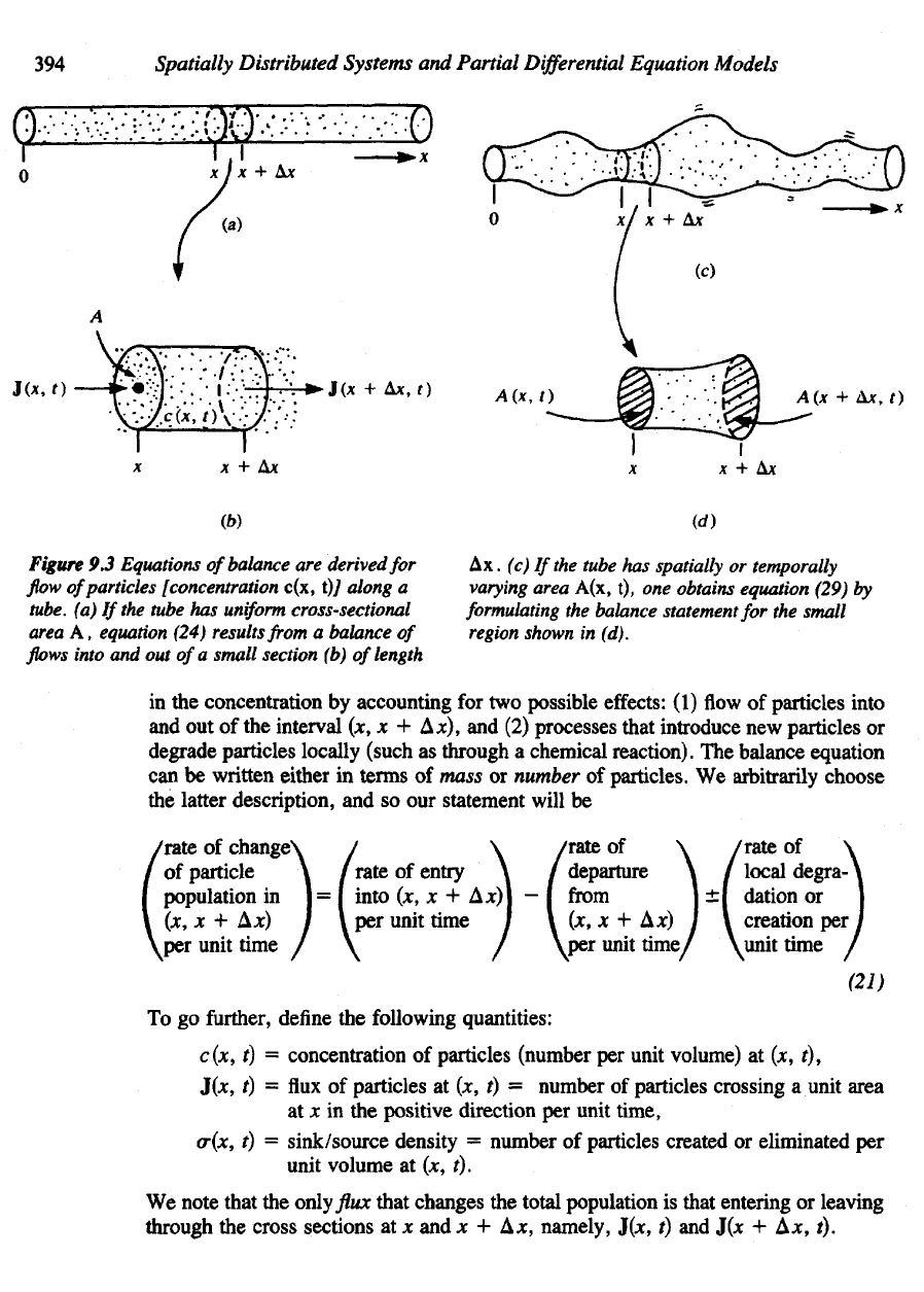
Figure
9.3
Equations
of
balance
are
derived
for
flow
of
particles [concentration
c(x,
t)7
along
a
tube,
(a)
If
the
tube
has
uniform
cross-sectional
area
A,
equation (24) results
from a
balance
of
flows
into
and out of a
small section
(b) of
length
Ax. (c)
If
the
tube
has
spatially
or
temporally
varying
area
A(x,
t), one
obtains equation (29)
by
formulating
the
balance statement
for the
small
region
shown
in
(d).
in
the
concentration
by
accounting
for two
possible
effects:
(1) flow of
particles
into
and
out of the
interval
(x, x +
Ax),
and (2)
processes
that introduce
new
particles
or
degrade
particles
locally
(such
as
through
a
chemical reaction).
The
balance equation
can
be
written
either
in
terms
of
mass
or
number
of
particles.
We
arbitrarily
choose
the
latter
description,
and so our
statement will
be
To go
further, define
the
following
quantities:
c(x,
t) =
concentration
of
particles
(number
per
unit volume)
at (x, t),
J(x,
t) = flux of
particles
at (x, t) =
number
of
particles
crossing
a
unit area
at x in the
positive
direction
per
unit time,
&(x,
t) =
sink/source density
=
number
of
particles
created
or
eliminated
per
unit
volume
at (x, t).
We
note that
the
only
flux
that changes
the
total
population
is
that entering
or
leaving
through
the
cross
sections
at x and x + Ax,
namely,
J(x,
t) and J(x + Ax, t).
Partial
Differential
Equations
and
Diffusion
in
Biological Settings
395
To now
translate (21) into
a
dimensionally correct equation,
it is
necessary
to
take into account
the
following quantiti
A
=
cross-sectional
area
of
tube
AV
=
volume
of
length element
A* = A
AJC.
Every term
in the
equation must have
the
same units
as the
terms
on the LHS of
(21): number
per
unit volume
per
unit time.
This leads
to the
following equation:
Note that since
c
depends
on two
variables,
its
derivative with respect
to time is a
partial derivative. Choosing
to
write equation (22)
in
terms
of x, the
coordinate
of
the
left
boundary
of the
interval,
is
entirely arbitrary since
we are
about
to
take
the
limit
AJC
-* 0.
We
observe that
a flux in the
positive
x
direction tends
to
contribute
to the net
population positively
at x but
negatively
at x + A*;
hence
the
signs
of the
terms
in
(22).
See
Figure
9.3(fr).
Now
dividing through
by A
AJC,
which
by
assumption
is
constant,
we
obtain
Taking
a
limit
of
this equation
as A*
—»
0,
that
is, as the
slice width gets vanist
ingly
small,
we
arrive
at a
local statement,
the
one-dimensional
balance equation,
The
minus sign
on
dj/dx stems
from
the
fact
that
the
finite
difference
in
(23)
has a
sign opposite
to
that
in the
definition
of a
derivative.
This
is the
basic
form
of the
balance
law
that
we
shall soon apply
to
numerous
specific
problems.
Before doing
so, we
will make
a
number
of
extensions
and
gen-
eral statements.
It is
possible
to
skip this material
and go on to
Section
9.4
without
loss
of
continuity.
9.3
OTHER VERSIONS
OF THE
CONSERVATION EQUATION
Tubular
Flow
We
shall
drop assumption
(2) and
consider
the
possibility
that
the
cross-sectional
area
of the
tube
may
vary over space
and
time.
To be
somewhat more formal,
we
take
the
following definitions:
By the
concentration c(x,
t) we
mean
a
quantity such
that