Gockenbach M.S. Partial Differential Equations. Analytical and Numerical Methods
Подождите немного. Документ загружается.

248
Chapter
6.
Heat flow
and
diffusion
The first
boundary condition yields
the
equation
while
the
second yields
Since
0 > 0,
these
equations reduce
to
and
respectively.
It
follows
that
the
only nonzero solutions
of
(6.22) correspond
to
and, moreover,
that
with
one of
these values
for A,
every function
of the
form
satisfies
(6.22).
Now,
are
linearly independent, which means
that
there
are two
independent
eigenfunc-
tions
for
each positive eigenvalue,
a
situation
we
have
not
seen before.
The
complete
list
of
eigenpairs
for the
negative second derivative operator, subject
to
periodic
boundary conditions,
is
We
know
that,
since
L
p
is
symmetric, eigenfunctions corresponding
to
distinct eigen-
values
are
orthogonal.
That
is, if
m
^
n,
then
is
orthogonal
to
both
Similarly,
248
Chapter
6.
Heat flow
and
diffusion
The
first boundary condition yields
the
equation
Cl
cos
(OC)
+
C2
sin
(OC)
=
Cl
cos
(OC)
-
C2
sin
(OC),
while
the
second yields
Since 8
>
0,
these equations reduce
to
C2
= ° or sin
(8C)
= °
and
Cl
= ° or sin
(OC)
= 0,
respectively.
It
follows
that
the
only nonzero solutions of (6.22) correspond
to
n
2
1l"2
A =
T'
n =
1,2,3,
...
,
and, moreover,
that
with one of these values for
A,
every function of
the
form
cos
(Ox)
or
sin
(Ox)
satisfies (6.22).
Now,
cos
(n;x)
and
sin (n;x)
are linearly independent, which means
that
there are two independent eigenfunc-
tions for each positive eigenvalue, a situation
we
have not seen before.
The
complete
list of eigenpairs for
the
negative second derivative operator, subject
to
periodic
boundary conditions,
is
Ao
= 0,
'Yo(x)
= 1;
n
2
1l"2
(n1l"x)
An
=
T'
'Yn(X)
= cos
-C-
, n =
1,2,3,
...
,
(6.23)
n
2
1l"2
(n1l"x)
An
=
T'
'¢n(X)
= sin
-C-
, n =
1,2,3,
....
We
know
that,
since Lp is symmetric, eigenfunctions corresponding
to
distinct eigen-
values are orthogonal.
That
is, if m
=f.
n,
then
(
m1l"X)
cos
-C-
is orthogonal
to
both
(
n1l"X)
.
(n1l"x)
cos
-C-
and
sm
-C-
.
Similarly,
.
(m1l"x)
sm
--
C
6.3.
Periodic
boundary
conditions
and the
full
Fourier
series
249
is
orthogonal
to
both
There
is no a
priori guarantee
that
the two
eigenfunctions corresponding
to
A
m
are
orthogonal
to
each other. However,
a
direct calculation shows this
to be
true.
We
can
also calculate
The
full
Fourier series
of a
function
/ €
C[—t,(\
is
given
by
where
We
will
show
in
Section
9.6
that
the
full
Fourier series
of a
C[—l,
I]
function
con-
verges
to it in the
mean-square sense (that
is,
that
the
sequence
of
partial Fourier
series converges
to the
function
in the
I/
2
-norm).
6.3.2
Solving
the BVP
using
the
full
Fourier
series
We
now
show
how to
solve
the BVP
(6.21) using
the
full
Fourier series. Since
the
method should
by now be
familiar,
we
leave
the
intermediate steps
to the
exercises.
We
write
the
(unknown) solution
of
(6.21)
as
where
the
coefficients
ao,
ai,
02,
• •
•,
&i,
&2,
• • • are to be
determined. Then
u
au-
tomatically satisfies
the
periodic boundary conditions.
The
full
Fourier series
for
—d
2
u/dx
2
is
given
by
(see
Exercise
6).
We
now
assume
that
the
source
function
/ has
full
Fourier series
6.3. Periodic boundary conditions
and
the full Fourier
series
249
is
orthogonal
to
both
(
nKX)
.
(nKX)
cos -e- and sm -e- .
There
is
no a priori guarantee
that
the two eigenfunctions corresponding to
Am
are
orthogonal
to
each other. However, a direct calculation shows this to be true.
We
can also calculate
(1,1)
=
2e,
bn,
'Yn)
=
('l/Jn,
'l/Jn)
=
e,
n =
1,2,3,
....
(6.24)
The lull Fourier series of a function
I E C[
-e,
£]
is
given by
where
1
ji
ao
=
2£
I(x)
dx,
-i
1
ji
(nKX)
a
n
=£
_/(x)cos
-£-
dx,
n=1,2,3, ... ,
(6.25)
b
n
=
~
ii/(X)
sin
(n;x)
dx,
n =
1,2,3,
..
..
We
will show in Section 9.6
that
the full Fourier series of a C[
-e,
£]
function con-
verges
to
it in the mean-square sense (that is,
that
the sequence of partial Fourier
series converges to the function in the
L
2
-norm).
6.3.2 Solving the
BVP
using
the full Fourier
series
We
now show how
to
solve the BVP (6.21) using the full Fourier series. Since
the
method should by now be familiar,
we
leave
the
intermediate steps
to
the exercises.
We
write the (unknown) solution of (6.21) as
00
u(x)
=
ao
+
2:=
{an
cos
(n;x)
+ b
n
sin
(n;x)
} ,
n=l
(6.26)
where the coefficients
ao,
aI,
a2,
... , b
1
,
b
2
, ...
are to be determined. Then u au-
tomatically satisfies the periodic boundary conditions. The full Fourier series for
-d
2
ujdx
2
is
given by
~u
00
{K,n
2
K2
(nKX)
K,n
2
K2
(nKX)}
-K,dx2(X)=~
an~cos
-e-
+bn~sin
-e-
(6.27)
(see Exercise 6).
We
now assume
that
the source function I has full Fourier series
00
I(x) =
C{)
+
2:=
{en
cos
(n;x)
+ d
n
sin
(n;x)
} ,
n=l
250
Chapter
6.
Heat flow
and
diffusion
where
the
coefficients
CQ,
ci,
C2,...,di,
fife?
• • •
can
be
determined explicitly, since
/
is
known. Then
the
differential
equation
implies
that
the
Fourier series
(6.27)
and
(6.28)
are
equal
and
hence
that
From
these equations,
we
deduce
first of all
that
the
source
function
/
must
satisfy
the
compatibility condition
in
order
for a
solution
to
exist.
If
(6.29)
holds, then
we
have
but
do
is not
determined
by the
differential
equation
or by the
boundary conditions
Therefore,
for any
CIQ,
is
a
solution
to
(6.21) (again, assuming
that
(6.29) holds).
Example
6.6.
We
consider
a
thin
gold
ring,
of
radius 1cm.
In the
above
notation,
then,
I
=
TT.
The
material properties
of
gold
are
p=l9.3g/cm
3
,
c =
0.129
Jf(gK),
K
=
3.17
W/(cmK).
We
assume that heat
energy
is
being
added
to the
ring
at the
rate
of
Since
250 Chapter
6.
Heat flow
and
diffusion
where
the
coefficients
Co,
Cl,
e2,
..•
,d
1
,
d
2
,
•..
can be determined explicitly, since f
is
known. Then the differential equation
~u
-r;,
dx
2
=
f(x)
implies
that
the
Fourier series (6.27) and (6.28) are equal and hence
that
0=
Co,
r;,n
2
7r
2
~an=en'
r;,n
2
7r
2
~bn=dn.
(6.28)
From these equations,
we
deduce first
of
all
that
the source function f must satisfy
the
compatibility condition
i£/(X)dX
= 0
(6.29)
in order for a solution
to
exist.
If
(6.29) holds, then
we
have
but
ao
is
not determined by the differential equation or by the boundary conditions.
Therefore, for any
ao,
is a solution
to
(6.21) (again, assuming
that
(6.29) holds).
Example
6.6.
We consider a thin gold ring,
of
radius 1em. In the
above
notation,
then,
f =
7r.
The material properties
of
gold
are
p=19.3g/cm
3
,
e=0.129J/(gK),
r;,=3.17W/(cmK).
We assume that heat energy is being added to the ring at the rate
of
Since
i:
f(x)
dx = 0,
A
graph
of
u is
shown
in
Figure 6.9.
We
emphasize that this solution
really
only
shows
the
variation
in the
temperature—the
true temperature
is
u(x)
+ C for
some
real
number
C. The
assumptions
above
do not
give enough information
to
determine
C;
we
would
have
to
know
the
amount
of
heat
energy
in the
ring
before
the
heat
source
f is
applied.
6.3. Periodic boundary conditions
and the
full Fourier
series
251
the
BVP
has a
solution.
We
write
(we
take
ao
= 0,
thus choosing
one
of
the
infinitely
many solutions).
We
then
have
Also,
where
Thus
(The value
of
CQ
is
already
known
to be
zero since
f
satisfies
the
compatibility con-
dition.)
Equating
the
last
two
series
yields
6.3. Periodic boundary conditions
and
the full Fourier
series
251
the
BVP
J2u
-I\, dx
2
=
f(x),
-7f < x <
7f,
u(
-7f) =
u(7f),
du du
dx
(-7f) =
dx
(7f)
has a solution. We write
00
u(x)
= L (an cos (nx) + b
n
sin
(nx))
n=l
{we
take
ao
= 0, thus choosing one
of
the infinitely
many
solutions}. We then have
-I\,
~~
(x) =
f:
(I\,n
2
a
n
cos (nx) +
I\,n
2
b
n
sin
(nx))
.
n=l
Also,
00
f (x) = L
(c
n
cos (nx) + d
n
sin
(nx))
,
n=l
where
1111"
C
n
= -
f(x)
cos (nx) dx = 0, n =
1,2,3,
...
,
7f
-11"
1111".
6(-1)n
d
n
= -
f(x)
sm
(nx)
dx
=
3'
n =
1,2,3,
....
7f
-11"
5n
(The value
of
Co
is already known to
be
zero since f satisfies the compatibility con-
dition.) Equating the last two series yields
Thus
2 C
n
I\,n
an = C
n
:::}
an =
-2
= 0, n =
1,2,3,
...
,
I\,n
2 d
n
12(-1)n
I\,n
b
n
= d
n
:::}
b
n
=
-2
=
10
5'
n =
1,2,3,
....
I\,n
I\,n
00
12(-1)n
.
u(x)
= L 10 5
sm
(nx).
n=l
I\,n
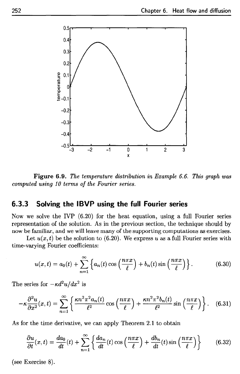
A graph
of
u is shown
in
Figure 6.9. We emphasize that this solution really only
shows the variation
in
the
temperature-the
true temperature is
u(x)
+ C for some
real number
C.
The assumptions
above
do
not
give enough information to determine
C;
we
would have to know the amount
of
heat energy
in
the ring before the heat
source f is applied.
252
Chapter
6.
Heat flow
and
diffusion
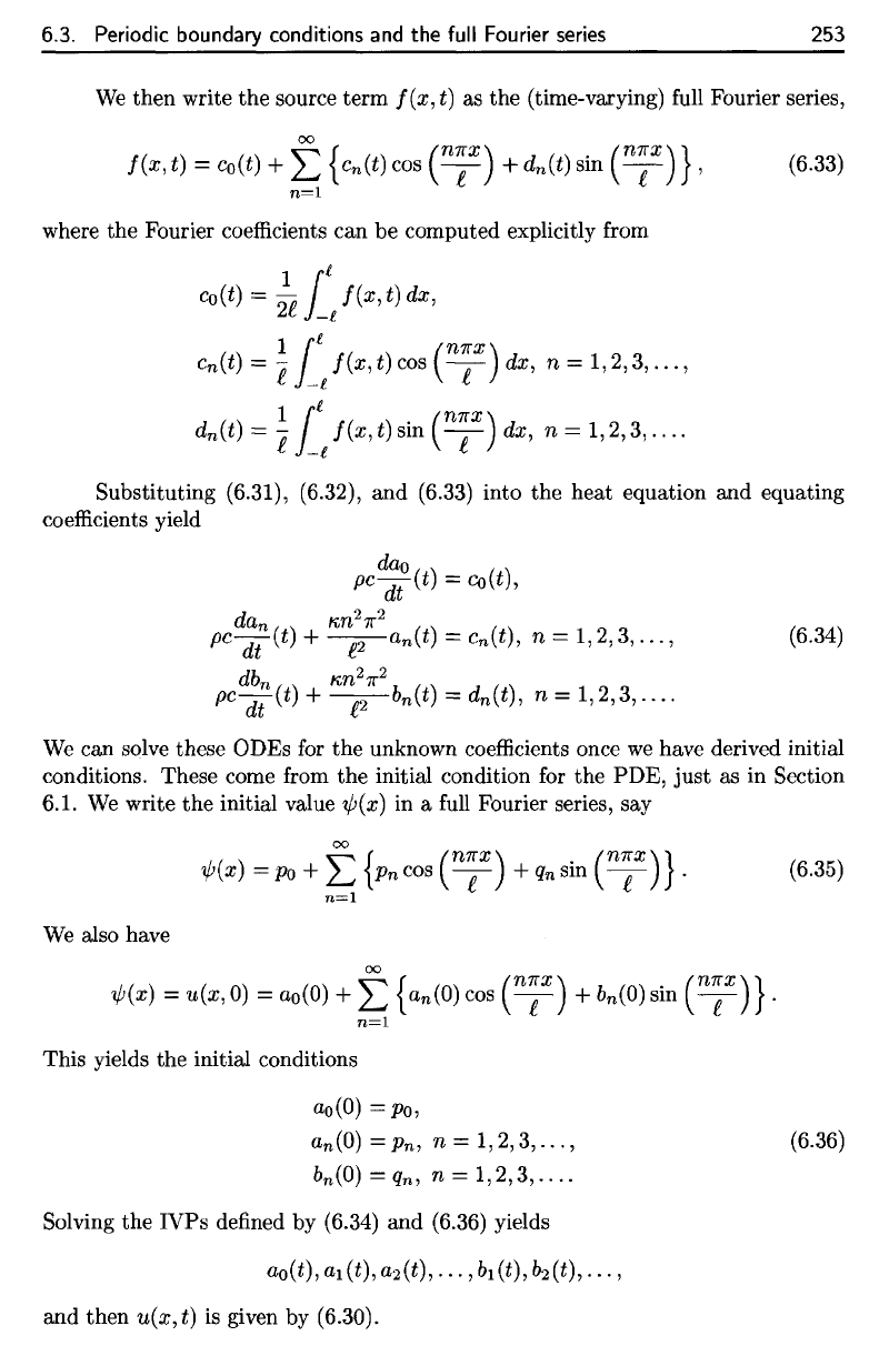
Figure
6.9.
The
temperature distribution
in
Example 6.6.
This
graph
was
computed
using
10
terms
of the
Fourier series.
6.3.3 Solving
the
IBVP
using
the
full Fourier
series
Now
we
solve
the
IVP
(6.20)
for the
heat
equation, using
a
full
Fourier series
representation
of the
solution.
As in the
previous section,
the
technique should
by
now
be
familiar,
and we
will
leave many
of the
supporting computations
as
exercises.
Let
u(x,
t)
be the
solution
to
(6.20).
We
express
u
as a
full
Fourier series with
time-varying
Fourier
coefficients:
The
series
for
—Kd?u/dx
2
is
As
for the
time derivative,
we can
apply Theorem
2.1 to
obtain
(see
Exercise
8).
252
Chapter
6.
Heat
flow
and
diffusion
0.5,.,.-----,,.-----.---r----r--.....----n
0.4
0.3
~
0.1
ca
Iii
0
a.
E
2-0.1
-0.2
-0.3
-0.4
-0.5
........
----''---
.........
--'----'---.&.--
.........
-3 -2
-1
0 2 3
x
Figure
6.9.
The
tempemture distribution in Example
6.6.
This gmph
was
computed using 10 terms
of
the Fourier series.
6.3.3
Solving
the I BVP
using
the
full
Fourier
series
Now
we
solve
the
IVP (6.20) for the heat equation, using a full Fourier series
representation of the solution.
As
in
the
previous section, the technique should
by
now be familiar, and
we
will leave many of the supporting computations as exercises.
Let
u(x, t) be
the
solution
to
(6.20).
We
express u as a full Fourier series with
time-varying Fourier coefficients:
00
u(x, t) =
ao(t)
+ L {an(t) cos
(n;x)
+
bn(t)
sin
(n;x)
} . (6.30)
n=l
The
series for -l'i.J2u/dx
2
is
(6.31)
As
for
the
time derivative,
we
can apply Theorem
2.1
to
obtain
au
dao
~
{dan (n1fx)
db
n
.
(n1fx)}
at
(x,
t) =
(jt(t)
+
~
dt
(t) cos -e- +
(jt(t)
sm -e-
(6.32)
(see Exercise 8).
6.3. Periodic boundary conditions
and the
full Fourier
series
253
We
then write
the
source term
/(#,£)
as the
(time-varying)
full
Fourier series,
where
the
Fourier
coefficients
can be
computed explicitly
from
Substituting
(6.31), (6.32),
and
(6.33) into
the
heat equation
and
equating
coefficients
yield
We
can
solve
these
ODEs
for the
unknown coefficients once
we
have derived
initial
conditions. These come
from
the
initial condition
for the
PDE, just
as in
Section
6.1.
We
write
the
initial value
ib(x]
in a
full
Fourier series,
sav
We
also have
This
yields
the
initial conditions
Solving
the
IVPs
defined
by
(6.34)
and
(6.36) yields
and
then
u(x,t)
is
given
by
(6.30),
6.3. Periodic boundary conditions
and
the full Fourier
series
253
We
then write
the
source term
f(x,
t) as the (time-varying) full Fourier series,
00
f(x,
t) = co(t) + L {cn(t) cos
(n;x)
+ dn(t) sin
(n;x)},
(6.33)
n=l
where the Fourier coefficients can be computed explicitly from
co(t) =
;e
il/(X,
t) dx,
III
(n7rx)
cn(t)
= e
_£
f(x,
t) cos -e- dx, n =
1,2,3,
...
,
dn(t) =
~
ill
f(x,
t) sin
(n;x)
dx, n =
1,2,3,
...
.
Substituting (6.31), (6.32), and (6.33) into the heat equation and equating
coefficients yield
dao
pCTt(t)
= eo(t),
dan
r;,n
2
7r
2
pc
dt (t) +
~an(t)
= cn(t), n =
1,2,3,
...
,
(6.34)
db
n
r;,n
2
7r
2
pcdt(t)
+
~bn(t)
= dn(t), n =
1,2,3,
....
We
can solve these ODEs for the unknown coefficients once
we
have derived initial
conditions. These come from the initial condition for the PDE, just as in Section
6.1.
We
write
the
initial value
1jJ(x)
in a full Fourier series, say
00
1jJ(x)
=
Po
+ L
{Pn
cos
(n;x)
+
qn
sin
(n;x)}
. (6.35)
n=l
We
also have
00
1jJ(x)
= u(x,
0)
=
ao(O)
+ L
{an(O)
cos
(n;x)
+
bn(O)
sin
(n;x)
} .
n=l
This yields the initial conditions
ao(O)
=
Po,
an(O)
=
Pn,
n =
1,2,3,
...
,
bn(O)
=
qn,
n =
1,2,3,
...
.
Solving
the
IVPs defined by (6.34) and (6.36) yields
ao(t),al(t),a2(t),
...
,b
1
(t),b
2
(t),
...
,
and
then u(x, t)
is
given by (6.30).
(6.36)
The
solutions
are
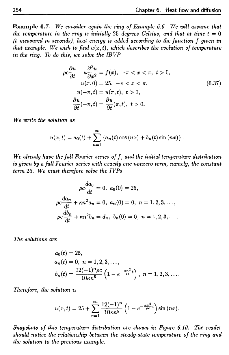
Snapshots
of
this temperature distribution
are
shown
in
Figure 6.10.
The
reader
should
notice
the
relationship between
the
steady-state temperature
of the
ring
and
the
solution
to the
previous example.
254
Chapter
6.
Heat
flow
and
diffusion
Example
6.7.
We
consider again
the
ring
of
Example 6.6.
We
will assume that
the
temperature
in the
ring
is
initially
25
degrees
Celsius,
and
that
at
time
t = 0
(t
measured
in
seconds), heat
energy
is
added
according
to the
function
f
given
in
that example.
We
wish
to findu(x,t],
which describes
the
evolution
of
temperature
in the
ring.
To do
this,
we
solve
the
IBVP
We
write
the
solution
as
We
already
have
the
full Fourier series
of
f,
and the
initial temperature distribution
is
given
by a
full Fourier series with exactly
one
nonzero
term,
namely,
the
constant
term
25. We
must
therefore
solve
the
IVPs
Therefore,
the
solution
is
254
Chapter
6.
Heat
flow
and
diffusion
Example
6.7.
We consider again the ring
of
Example 6.6. We will assume that
the temperature
in
the ring is initially
25
degrees Celsius, and that at time t = °
(t measured
in
seconds), heat energy is added according to the function f given
in
that example. We wish to find
u(x,
t),
which describes the evolution
of
temperature
in
the ring.
To
do
this,
we
solve the
IBVP
{)u
{)2U
pc
{)t
-,.;,
{)x
2
=
f(x),
-Jr
< x <
Jr,
t>
0,
u(x,O) = 25,
-Jr
< x <
Jr,
(6.37)
u(
-Jr,
t) =
u(Jr,
t), t > 0,
{)U
{)u
{)t
(-Jr,t)
=
{)t
(Jr,t), t >
0.
We write the solution
as
00
u(x,
t) = ao(t) + L {an(t)
cos
(nx) + bn(t) sin
(nx)}.
n=l
We already have the full Fourier series
of
f,
and the initial temperature distribution
is given by a full Fourier series with exactly one nonzero term, namely, the constant
term 25. We
must
therefore solve the
IVPs
da
o
pCTt
=
0,
ao(O)
= 25,
dan 2 ( )
pc dt +,.;,n an =
0,
an ° =
0,
n = 1,2,3,
...
,
db
n
2 ( )
pCTt+,.;,nbn=dn,
bnO
=0,
n=1,2,3,
....
The solutions
are
ao(t) = 25,
an(t) =
0,
n = 1,2,3,
...
,
12(-1)n
pC
(
_I<n
2t
)
bn(t) = 5 1 - e
pc
,n
=
1,2,3,
....
10,.;,n
Therefore, the solution is
~
12(-1)n
( 1<,,2 )
u(x,
t) =
25
+
~
10,.;,n
5
1 -
e-pc-t
sin
(nx).
n=l
Snapshots
of
this temperature distribution
are
shown
in
Figure 6.10. The reader
should notice the relationship between the steady-state temperature
of
the ring and
the solution to the previous example.
6.3. Periodic boundary conditions
and the
full Fourier
series
255
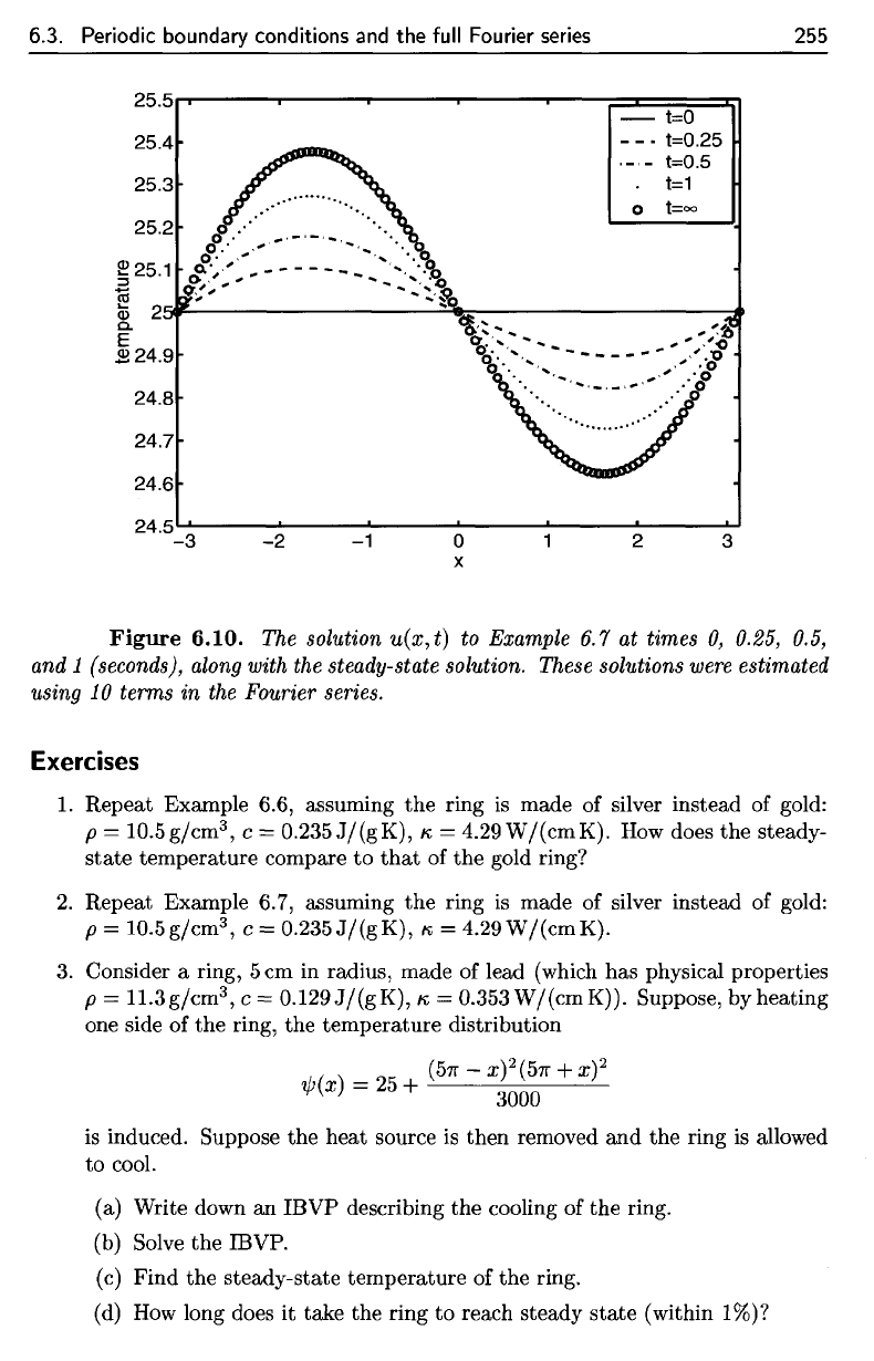
Figure
6.10.
The
solution
w(x,t)
to
Example
6.7 at
times
0,
0.25, 0.5,
and
1
(seconds),
along
with
the
steady-state solution.
These
solutions
were
estimated
using
10
terms
in the
Fourier series.
Exercises
1.
Repeat Example 6.6, assuming
the
ring
is
made
of
silver instead
of
gold:
p
=
10.5
g/cm
3
,
c =
0.235
J/(gK),
«
=
4.29
W/(cm
K). How
does
the
steady-
state
temperature compare
to
that
of the
gold ring?
2.
Repeat Example 6.7, assuming
the
ring
is
made
of
silver instead
of
gold:
p
=
10.5g/cm
3
,
c =
0.235
J/(gK),
K =
4.29W/(cmK).
3.
Consider
a
ring,
5cm
in
radius, made
of
lead
(which
has
physical properties
p
=
11.3
g/cm
3
,
c =
0.129 J/(gK),
«
=
0.353
W/(cm
K)).
Suppose,
by
heating
one
side
of the
ring,
the
temperature distribution
is
induced. Suppose
the
heat source
is
then removed
and the
ring
is
allowed
to
cool.
(a)
Write down
an
IBVP
describing
the
cooling
of the
ring.
(b)
Solve
the
IBVP.
(c)
Find
the
steady-state temperature
of the
ring.
(d)
How
long does
it
take
the
ring
to
reach
steady
state
(within
1%)?
6.3. Periodic boundary conditions
and
the full Fourier
series
25.5
25.4
25.3
25.2
~25.1
:::J
~
2
Q)
0.
E
224.9
24.8
24.7
24.6
24.5
-3 -2
-1
-
t=O
-
_.
t=O.25
t=O.5
t=1
o
t=oo
~,~.......
,":t)
0.'"
.......
__
"'--
o
x
a - -
..
'"
,,'~
o·
°
0
',....
- - - -
....
v
....
:
..
","
-,-
,~'~".'.~·l
2 3
255
Figure
6.10.
The solution
u(x,
t) to Example 6.7 at times
0,
0.25, 0.5,
and
1 (seconds), along with the steady-state solution. These solutions were estimated
using
10
terms in the Fourier series.
Exercises
1.
Repeat Example 6.6, assuming
the
ring
is
made of silver instead of gold:
p =
10.5g/cm
3
,
c = O.235J/(gK), K, =
4.29W/(cmK).
How does
the
steady-
state
temperature compare
to
that
of
the
gold ring?
2.
Repeat Example 6.7, assuming
the
ring
is
made of silver instead of gold:
p = IO.5g/cm3, c =
O.235J/(gK),
K, =
4.29W/(cmK).
3. Consider a ring, 5 cm in radius, made of lead (which has physical properties
p =
11.3g/cm
3
,
c = O.129J/(gK), K, = O.353W/(cmK)). Suppose, by heating
one side of
the
ring, the
temperature
distribution
is induced. Suppose
the
heat source
is
then
removed
and
the
ring
is
allowed
to
cool.
(a) Write down
an
IBVP
describing the cooling of
the
ring.
(b) Solve
the
IBVP.
(c)
Find
the
steady-state
temperature
of
the
ring.
(d) How long does
it
take the ring
to
reach steady
state
(within 1%)?
(c)
by
analogy
to the
compatibility condition given
in the
Predholm
alter-
native.
8.
Show
that
the
Fourier series representation (6.32)
follows
from
(6.30)
and
Theorem
2.1.
6.4
Finite
element methods
for the
heat equation
To
apply
the
Fourier series method
to the
heat equation,
we
used
the
familiar
eigenfunctions
to
represent
the
spatial
variation
of the
solution, while allowing
the
Fourier
coefficients
to
depend
on
time.
We
then
found
the
values
of
these Fourier
coefficients
by
solving ODEs.
We can use the finite
element method
in an
analogous
fashion.
We use finite
element functions
to
approximate
the
spatial variation
of the
solution, while
the
coefficients
in the
representation depend
on
time.
We end up
with
a
system
of
ODEs whose solution yields
the
unknown
coefficients.
256
Chapter
6.
Heat
flow
and
diffusion
4.
Consider
the
lead ring
of the
previous exercise. Suppose
the
temperature
is
a
constant
25
degrees Celsius,
and an
(uneven) heat source
is
applied
to the
ring.
If the
heat source delivers heat energy
to the
ring
at a
rate
of
how
long does
it
take
for the
temperature
at the
hottest
part
of the
ring
to
rpa.rh
30
HPCTTPPS
("Iplsiiifi?
5.
(a)
Show
that
L
p
is
symmetric.
(b)
Show
that
L
p
does
not
have
any
negative eigenvalues.
6.
Assuming
that
u is a
smooth
function
defined
on
[—£,
£],
the
full
Fourier series
of
u is
given
by
(6.26),
and u
satisfies periodic boundary conditions, show
that
the
full
Fourier series
of
—d^u/dx
2
is
given
by
(6.27).
7.
Justify
the
compatibility condition (6.29)
(a)
by
physical reasoning (assume
that
(6.21) models
a
steady-state temper-
ature distribution
in a
circular
ring);
(b)
by
using
the
differential
equation
256
Chapter
6.
Heat
flow
and
diffusion
4.
Consider the lead ring of
the
previous exercise. Suppose the temperature
is
a constant
25
degrees Celsius, and
an
(uneven) heat source
is
applied
to
the
ring.
If
the heat source delivers heat energy to
the
ring
at
a
rate
of
f(x)
=
1-
~~
Wjcm
3
,
how long does it take for
the
temperature
at
the
hottest
part
of the ring
to
reach 30 degrees Celsius?
5.
(a) Show
that
Lp
is
symmetric.
(b) Show
that
Lp does not have any negative eigenvalues.
6. Assuming
that
u
is
a smooth function defined on [-£,
£l,
the full Fourier series
of
u is given by (6.26), and u satisfies periodic boundary conditions, show
that
the
full Fourier series of
-d
2
ujdx
2
is
given by (6.27).
7.
Justify
the
compatibility condition (6.29)
(a) by physical reasoning (assume
that
(6.21) models a steady-state temper-
ature distribution in a circular ring);
(b) by using
the
differential equation
~u
- dx
2
(x) =
f(x),
-£
< x <
£,
and
the
periodic boundary conditions
to
compute
i:
f(x)dx;
(c)
by analogy to the compatibility condition given in the Fredholm alter-
native.
8.
Show
that
the Fourier series representation (6.32) follows from (6.30) and
Theorem 2.1.
6.4 Finite element methods for the heat equation
To apply
the
Fourier series method
to
the
heat equation,
we
used the familiar
eigenfunctions
to
represent
the
spatial variation of
the
solution, while allowing the
Fourier coefficients to depend on time.
We
then found the values of these Fourier
coefficients by solving ODEs.
We
can use the finite element method in an analogous
fashion.
We
use finite element functions
to
approximate
the
spatial variation of the
solution, while
the
coefficients in
the
representation depend on time.
We
end up
with a system of ODEs whose solution yields the unknown coefficients.
This
is the
weak
form
of the
IBVP.
To get an
approximate solution,
we
apply
the
Galerkin
method with approximating
subspace
Sn
=
{p
'•
[0,
f\
—>
R
: p is
continuous
and
piecewise linear,
p(0)
=
p(t]
= 0}
=
span{0i,0
2
,...,0n-i},
where
the
piecewise linear
functions
are
defined
on the
grid
0 =
XQ
<
x\
< • • • <
x
n
= t and
{0i,
02?
• •
•,
0n-i}
is the
standard basis
defined
in the
previous chapter.
For
each
t, the
function
u(-,t]
must
lie in
S
n
,
that
is,
6.4.
Finite
element methods
for the
heat equation
257
We
will consider again
the
following
IBVP:
We
begin
by
deriving
the
weak
form
of the
IBVP,
following
the
pattern
of
Section
5.4.2
(multiply
the
differential
equation
by a
test
function
and
integrate
by
parts
on
the
left).
In the
following
calculation,
V is the
same space
of
test
functions used
for
the
problem
in
statics:
We
have
We
integrate
by
parts
in the
second term
on the
left;
the
boundary term
from
integration
by
parts vanishes because
of the
boundary conditions
on the
test
function
v(x),
and we
obtain
6.4.
Finite
element
methods
for
the
heat
equation
257
We
will consider again the following IBVP:
{)u
{)2U
pc
{)t
- /'i,
{)x
2
=
I(x,
t), ° < x <
e,
t >
to,
u(x,
to)
=
'Ij!(x),
° < x <
e,
(6.38)
u(O,
t) = 0, t >
to,
u(e,t) = 0, t >
to.
We
begin by deriving the weak form of the IBVP, following the
pattern
of Section
5.4.2 (multiply the differential equation by a test function and integrate by
parts
on the left).
In
the following calculation, V
is
the
same space of test functions used
for the problem in statics:
V =
cb[o,e].
We
have
{)u
{)2u
pc
{)t
- /'i,
{)x
2
=
I(x,
t), ° < x < t, t >
to
{)u
{)2U
=}
pc
{)t
(x, t)v(x) - /'i,
{)x
2
(x, t)v(x) =
I(x,
t)v(x), ° < x < t,
t>
to,
v E V
=}
1£
{pc
~~
(x, t)v(x) - /'i,
~:~
(x,
t)v(x)}
dx =
1£
I(x,
t)v(x) dx,
t>
to,
v E
V.
We
integrate by
parts
in the second
term
on the left;
the
boundary
term
from
integration by parts vanishes because of the boundary conditions on the test function
vex),
and
we
obtain
1£
{pc
~~
(x, t)v(x) + /'i,
~~
(x, t)
::
(x) } dx
£
=
10
I(x,
t)v(x) dx,
t>
to
for all v E
V.
This
is
the
weak form of the IBVP. To get
an
approximate solution,
we
apply the
Galerkin method with approximating subspace
Sn =
{p:
[0,
e]
-+
R : p
is
continuous and piecewise linear,
p(O)
=
pee)
=
O}
= span{¢h,CP2,
...
,CPn-d,
where the piecewise linear functions are defined on the grid ° =
Xo
<
Xl
< ... <
xn
= t and
{CPI,
CP2,
... ,
CPn-l}
is
the
standard
basis defined in
the
previous chapter.
For each t,
the
function u(·, t) must lie in Sn,
that
is,
n-l
un(x, t) = L
D:i(t)cpi(X).
(6.39)
i=l