Goldreich O. Computational Complexity. A Conceptual Perspective

Подождите немного. Документ загружается.

CUUS063 main CUUS063 Goldreich 978 0 521 88473 0 March 31, 2008 18:49

5.1. GENERAL PRELIMINARIES AND ISSUES

space complexity of search problems is deﬁned analogously. Speciﬁcally, the standard

deﬁnition

of space complexity (see §1.2.3.5) refers to the number of cells of the work-tape

scanned by the machine on each input. We prefer, however, an alternative deﬁnition,

which provides a more accurate account of the actual storage. Speciﬁcally, the

binary

space complexity

of a computation refers to the number of bits that can be stored in these

cells, thus multiplying the number of cells by the logarithm of the ﬁnite set of work-tape

symbols of the machine.

The difference between the two aforementioned deﬁnitions is mostly immaterial be-

cause it amounts to a constant factor and we will usually discard such factors. Neverthe-

less, aside from being conceptually right, using the deﬁnition of binary space complexity

facilitates some technical details (because the number of possible “instantaneous con-

ﬁgurations” is explicitly upper-bounded in terms of binary space complexity, whereas

its relation to the standard deﬁnition depends on the machine in question). Toward such

applications, we also count the ﬁnite state of the machine in its space complexity. Further-

more, for the sake of simplicity, we also assume that the machine does not scan the input

tape beyond the boundaries of the input, which are indicated by special symbols.

We stress that individual locations of the (read-only) input-tape (or device) may be

read several times. This is essential for many algorithms that use a sub-linear amount of

space (because such algorithms may need to scan their input more than once while they

cannot afford copying their input to their storage device). In contrast, rewriting on (the

same location of) the write-only output-tape is inessential, and in fact can be eliminated

at a relatively small cost (see Exercise 5.2).

Summary. Let us compile a list of the foregoing conventions. As stated, the ﬁrst two

items on the list are of crucial importance, while the rest are of technical nature (but do

facilitate our exposition).

1. Space complexity discards the use of the input and output devices.

2. The input device is read-only and the output device is write-only.

3. We will usually refer to the binary space complexity of algorithms, where the binary

space complexity of a machine M that uses the alphabet , ﬁnite state set Q, and has

standard space complexity S

is deﬁned as (log

|Q|) +(log

||) · S

. (Recall that

measures the number of cells of the temporary storage device that are used by M

during the computation.)

4. We will assume that the machine does not scan the input device beyond the boundaries

of the input.

5. We will assume that the machine does not rewrite to locations of its output device

(i.e., it writes to each cell of the output device at most once).

5.1.2. On the Minimal Amount of Useful Computation Space

Bearing in mind that one of our main objectives is identifying natural subclasses of P,we

consider the question of what is the minimal amount of space that allows for meaningful

computations. We note that regular sets [123, Chap. 2] are decidable by constant-space

We note that, unlike in the context of time complexity, linear speedup (as in Exercise 4.12) does not seem to

represent an actual saving in space resources. Indeed, time can be sped up by using stronger hardware (i.e., a Turing

machine with a bigger work alphabet), but the actual space is not really affected by partitioning it into bigger chunks

(i.e., using bigger cells). This fact is demonstrated when considering the binary space complexity of the two machines.

As indicated by Exercise 5.1, little is lost by this natural assumption.

145

CUUS063 main CUUS063 Goldreich 978 0 521 88473 0 March 31, 2008 18:49

SPACE COMPLEXITY

Turing machines and that this is all that the latter can decide (see, e.g., [123, Sec. 2.6]). It

is tempting to say that sub-logarithmic space machines are not more useful than constant-

space machines, because it seems impossible to allocate a sub-logarithmic amount of

space. This wrong intuition is based on the presumption that the allocation of a non-

constant amount of space requires explicitly computing the length of the input, which in

turn requires logarithmic space. However, this presumption is wrong: The input itself (in

case it is of a proper form) can be used to determine its length (and/or the allowed amount

of space).

In fact, for (n) = log log n, the class DSPACE(O()) is a proper superset of

SPACE(O(1)); see Exercise 5.3. On the other hand, it turns out that double-logarithmic

space is indeed the smallest amount of space that is more useful than constant space (see

Exercise 5.4); that is, for (n) = log log n, it holds that D

SPACE(o()) = DSPACE(O(1)).

In spite of the fact that some non-trivial things can be done in sub-logarithmic space

complexity, the lowest space-complexity class that we shall study in depth is logarithmic

space (see Section 5.2). As we shall see, this class is the natural habitat of several

fundamental computational phenomena.

A parenthetical comment (or a side lesson). Before proceeding, let us highlight the fact

that a naive presumption about arbitrary algorithms (i.e., that the use of a non-constant

amount of space requires explicitly computing the length of the input) could have led us

to a wrong conclusion. This demonstrates the danger in making “reasonable looking” (but

unjustiﬁed) presumptions about arbitrary algorithms. We need to be fully aware of this

danger whenever we seek impossibility results and/or complexity lower bounds.

5.1.3. Time Versus Space

Space complexity behaves very different from time complexity and indeed different

paradigms are used in studying it. One notable example is provided by the context of

algorithmic composition, discussed next.

5.1.3.1. Two Composition Lemmas

Unlike time, space can be reused; but, on the other hand, intermediate results of a com-

putation cannot be recorded for free. These two conﬂicting aspects are captured in the

following composition lemma.

Lemma 5.1 (naive composition): Let f

: {0, 1}

∗

→{0, 1}

∗

and f

: {0, 1}

∗

{0, 1}

∗

→{0, 1}

∗

be computable in space s

and s

, respectively.

Then f deﬁned

by f (x)

def

= f

(x, f

(x)) is computable in space s such that

s(n) = max(s

(n), s

(n + (n))) + (n) + δ(n),

Indeed, for this approach to work, we should be able to detect the case that the input is not of the proper form

(and do so within sub-logarithmic space).

Here (and throughout the chapter) we assume, for simplicity, that all complexity bounds are monotonically non-

decreasing. Another minor inaccuracy (in the text) is that we stated the complexity of the algorithm that computes f

in a somewhat non-standard way. Recall that by the standard convention, the complexity of an algorithm should be

stated in terms of the length of its input, which in this case is a pair (x, y) that may be encoded as a string of length

|x |+|y|+2log

|x | (but not as a string of length |x|+|y|). An alternative convention is to state the complexity of

such computations in terms of the length of both parts of the input (i.e., have s : N × N → N rather than s : N → N),

but we did not do this either.

146

CUUS063 main CUUS063 Goldreich 978 0 521 88473 0 March 31, 2008 18:49

5.1. GENERAL PRELIMINARIES AND ISSUES

f(x)

f (x)

counters

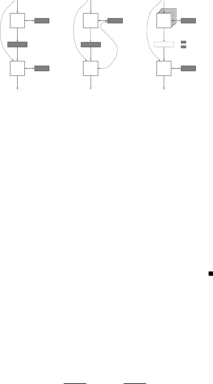
Figure 5.1: Three composition methods for space-bounded computation. The leftmost ﬁgure shows

the trivial composition (which just invokes A

and A

without attempting to economize storage), the

middle ﬁgure shows the naive composition (of Lemma 5.1), and the rightmost ﬁgure shows the emulative

composition (of Lemma 5.2). In all ﬁgures the ﬁlled rectangles represent designated storage spaces. The

dotted rectangle represents a virtual storage device.

where (n) = max

x∈{0,1}

{| f

(x)|} and δ(n) = O(log((n) + s

(n + (n)))) =

o(s(n)).

Lemma 5.1 is useful when  is relatively small, but in many cases   max(s

, s

). In

these cases, the following composition lemma is more useful.

Proof: Indeed, f (x) is computed by ﬁrst computing and storing f

(x), and then

reusing the space (used in the ﬁrst computation) when computing f

(x, f

(x)).

This explains the dominant terms in s(n); that is, the term max(s

(n), s

(n + (n)))

accounts for the computations themselves (which reuse the same space), whereas

the term (n) accounts for storing the intermediate result (i.e., f

(x)). The extra term

is due to implementation details. Speciﬁcally, the same storage device is used both

for storing f

(x) and for providing work-space for the computation of f

, which

means that we need to maintain our location on each of these two parts (i.e., the

location of the algorithm (that computes f

)on f

(x) and its location on its own

work space). (See further discussion at end of the proof of Lemma 5.2.) The extra

O(1) term accounts for the overhead involved in emulating two algorithms.

Lemma 5.2 (emulative composition): Let f

, f

, s

,and f beasinLemma5.1.

Then f is computable in space s such that

s(n) = s

(n) + s

(n + (n)) + O(log(n + (n))) + δ(n),

where δ(n) = O(log(s

(n) + s

(n + (n)))) = o(s(n)).

The alter native compositions are depicted in Figure 5.1 (which also shows the most

straightforward composition that makes no attempt to economize space).

Proof: The idea is avoiding the storage of the temporary value of f

(x) by computing

each of its bits (“on the ﬂy”) whenever this bit is needed for the computation of

147

CUUS063 main CUUS063 Goldreich 978 0 521 88473 0 March 31, 2008 18:49

SPACE COMPLEXITY

. That is, we do not start by computing f

(x), but rather start by computing

(x, f

(x)) although we do not have some of the bits of the relevant input (i.e., the

bits of f

(x)). The missing bits will be computed (and recomputed) whenever we

need them in the computation of f

(x, f

(x)). Details follow.

Let A

and A

be the algorithms (for computing f

and f

, respectively) guar-

anteed in the hypothesis.

Then, on input x ∈{0, 1}

, we invoke algorithm A

(for

computing f

). Algorithm A

is invoked on a virtual input, and so when emulating

each of its steps we should provide it with the relevant bit. Thus, we should also

keep track of the location of A

on the imaginary (virtual) input-tape. Whenever A

seeks to read the i

bit of its input, where i ∈ [n + (n)], we provide A

with this bit

by reading it from x if i ≤ n and invoke A

(x) otherwise. When invoking A

(x)we

provide it with a virtual output-tape, which means that we get the bits of its output

one by one and do not record them anywhere. Instead, we count until reaching the

(i − n)

output-bit, which we then pass to A

(as the i

bit of x, f

(x)).

Note that while invoking A

(x), we suspend the execution of A

but keep its

current conﬁguration such that we can resume the execution (of A

) once we get

the desired bit. Thus, we need to allocate separate space for the computation of A

and for the computation of A

. In addition, we need to allocate separate storage for

maintaining the aforementioned counters (i.e., we use log

(n + (n)) bits to hold the

location of the input-bit currently read by A

, and log

(n) bits to hold the index of

the output-bit currently produced in the current invocation of A

A ﬁnal (and tedious) issue is that our description of the composed algorithm

refers to two storage devices, one for emulating the computation of A

and the other

for emulating the computation of A

. The issue is not the fact that the storage (of

the composed algorithm) is partitioned between two devices, but rather that our

algorithm uses two pointers (one per each of the two storage devices). In contrast,

a (“fair”) composition result should yield an algorithm (like A

and A

) that uses a

single storage device with a single pointer to locations on this device. Indeed, such

an algorithm can be obtained by holding the two original pointers in memory; the

additional δ(n) ter m accounts for this additional storage.

Reﬂection. The algorithm presented in the proof of Lemma 5.2 is wasteful in ter ms of

time: it recomputes f

(x) again and again (i.e., once per each access of A

to the second

part of its input). Indeed, our aim was economizing on space and not on time (and the two

goals may be conﬂicting (see, e.g., [59, Sec. 4.3])).

5.1.3.2. An Obvious Bound

The time complexity of an algorithm is essentially upper bounded by an exponential

function in its space complexity. This is due to an upper bound on the number of pos-

sible instantaneous “conﬁgurations” of the algorithm (as formulated in the proof of

Theorem 5.3), and to the fact that if the computation passes through the same

conﬁguration twice then it must loop forever.

Theorem 5.3: If an algorithm A has binar y space complexity s and halts on every

input then it has time complexity t such that t (n) ≤ n · 2

s(n)+log

s(n)

We assume, for simplicity, that algorithm A

never rewrites on (the same location of) its write-only output-tape.

As shown in Exercise 5.2, this assumption can be justiﬁed at an additive cost of O(log (n)). Alternatively, the idea

presented in Exercise 5.2 can be incorporated directly in the current proof.

148

CUUS063 main CUUS063 Goldreich 978 0 521 88473 0 March 31, 2008 18:49

5.1. GENERAL PRELIMINARIES AND ISSUES

Note that for s(n) = (log n), the factor of n can be absorbed by 2

O(s(n))

, and so we

may just write t(n) = 2

O(s(n))

. Indeed, throughout this chapter (as in most of this book),

we will consider only algorithms that halt on every input (see Exercise 5.5 for further

discussion).

Proof: The proof refers to the notion of an instantaneous conﬁguration (in a com-

putation). Before starting, we warn the reader that this notion may be given different

deﬁnitions, each tailored to the application at hand. All these deﬁnitions share the

desire to specify variable information that together with some ﬁxed information

determines the next step of the computation being analyzed. In the current proof,

we ﬁx an algorithm A and an input x, and consider as variable the contents of the

storage device (e.g., work-tape of a Turing machine as well as its ﬁnite state) and the

machine’s location on the input device and on the storage device. Thus, an

instanta-

neous conﬁguration of

A(x) consists of the latter three objects (i.e., the contents of

the storage device and a pair of locations), and can be encoded by a binar y string of

length (|x|) = s(|x|) + log

|x|+log

s(|x|).

The key observation is that the computation A(x) cannot pass through the same

instantaneous conﬁguration twice, because otherwise the computation A(x) passes

through this conﬁguration inﬁnitely many times, which means that this computation

does not halt. This observation is justiﬁed by noting that the instantaneous conﬁgu-

ration, together with the ﬁxed information (i.e., A and x), determines the next step

of the computation. Thus, whatever happens (i steps) after the ﬁrst time that the

computation A (x) passes through conﬁguration γ will also happen (i steps) after

the second time that the computation A(x) passes through γ .

By the foregoing observation, we infer that the number of steps taken by A

on input x is at most 2

(|x |)

, because otherwise the same conﬁguration will appear

twice in the computation (which contradicts the halting hypothesis). The theorem

follows.

5.1.3.3. Subtleties Regarding Space-Bounded Reductions

Lemmas 5.1 and 5.2 sufﬁce for the analysis of the effect of many-to-one reductions in the

context of space-bounded computations. (By a many-to-one reduction of the function f to

the function g, we mean a mapping π such that for every x it holds that f (x) = g(π(x)).)

1. (In the spirit of Lemma 5.1:) If f is reducible to g via a many-to-one reduction that

can be computed in space s

, and g is computable in space s

, then f is computable in

space s such that s(n) = max(s

(n), s

((n))) + (n) + δ(n), where (n) denotes the

maximum length of the image of the reduction when applied to some n-bit string and

δ(n) = O(log((n) +s

((n)))) = o(s(n)).

2. (In the spirit of Lemma 5.2:) For f and g as in Item 1, it follows that f is com-

putable in space s such that s(n) = s

(n) + s

((n)) + O(log (n)) +δ(n), where

δ(n) = O(log(s

(n) + s

((n)))) = o(s(n)).

Here we rely on the fact that s is the binary space complexity (and not the standard space complexity); see

summary item 3 in Section 5.1.1.

This is indeed a special case of the setting of Lemmas 5.1 and 5.2 (obtained by letting f

= π and f

(x , y) = g(y)).

However, the results claimed for this special case are better than those obtained by invoking the corresponding lemma

(i.e., s

is applied to (n) rather than to n + (n)).

149

CUUS063 main CUUS063 Goldreich 978 0 521 88473 0 March 31, 2008 18:49

SPACE COMPLEXITY

Note that by Theorem 5.3, it holds that (n) ≤ 2

(n)+log

(n)

· n. We stress the fact that 

is not upper-bounded by s

itself (as in the analogous case of time-bounded computation),

but rather by exp(s

Things get much more complicated when we turn to general (space-bounded) reduc-

tions, especially when referring to general reductions that make a non-constant number of

queries. A preliminary issue is deﬁning the space complexity of general reductions (i.e.,

of oracle machines). In the standard deﬁnition, the length of the queries and answers is

not counted in the space complexity, but the queries of the reduction (resp., answers given

to it) are written on (resp., read from) a special device that is write-only (resp., read-only)

for the reduction (and read-only (resp., write-only) for the invoked oracle). Note that these

convention are analogous to the conventions regarding input and output (as well as ﬁt the

deﬁnitions of space-bounded many-to-one reductions that were outlined in the foregoing

items).

The foregoing conventions sufﬁce for deﬁning general space-bounded reductions. They

also sufﬁce for obtaining appealing composition results in some cases (e.g., for reductions

that make a single query or, more generally, for the case of non-adaptive queries). But

more difﬁculties arise when seeking composition results for general reductions, which may

make several adaptive queries (i.e., queries that depend on the answers to prior queries).

As we shall show next, in this case it is essential to upper-bound the length of every query

and/or every answer in terms of the length of the initial input.

Teaching note: The rest of the discussion is quite advanced and laconic (but is inessential to

the rest of the chapter).

Recall that the complexity of the algorithm resulting from the composition of an oracle

machine and an actual algorithm (which implements the oracle) depends on the length

of the queries made by the oracle machine. For example, the space complexity of the

foregoing compositions, which referred to single-query reductions, had an s

((n)) term

(where (n) represents the length of the query). In general, the length of the ﬁrst query is

upper-bounded by an exponential function in the space complexity of the oracle machine,

but the same does not necessarily hold for subsequent queries, unless some conventions

are added to enforce it. For example, consider a reduction that, on input x and access to

an oracle f such that |f (z)|=2|z|, invokes the oracle |x| times, where each time it uses

as a query the answer obtained to the previous query. This reduction uses constant space,

but produces queries that are exponentially longer than the input, whereas the ﬁrst query

of any constant-space reduction has length that is linear in its input. This problem can

be resolved by placing explicit bounds on the length of the queries that space-bounded

reductions are allowed to make; for example, we may bound the length of all queries by

the obvious bound that holds for the length of the ﬁrst query (i.e., a reduction of space

complexity s is allowed to make queries of length at most 2

s(n)+log

s(n)

· n).

With the aforementioned convention (or restriction) in place, let us consider the com-

position of general space-bounded reductions with a space-bounded implementation of

the oracle. Speciﬁcally, we say that a reduction is ( , 



)-restricted if, on input x, all oracle

queries are of length at most (|x|) and the corresponding oracle answers are of length

at most 



(|x|). It turns out that naive composition (in the spirit of Lemma 5.1) remains

useful, whereas the emulative composition of Lemma 5.2 breaks down (in the sense that

it yields very weak results).

150

CUUS063 main CUUS063 Goldreich 978 0 521 88473 0 March 31, 2008 18:49

5.1. GENERAL PRELIMINARIES AND ISSUES

1. Following Lemma 5.1, we claim that if  can be solved in space s

when given

(, 



)-restricted oracle access to 



and 



is solvable is space s

, then  is

solvable in space s such that s(n) = s

(n) + s

((n)) + (n) + 



(n) + δ(n), where

δ(n) = O(log((n) +



(n) + s

((n)))) = o(s(n)). This claim is proved by

using a naive emulation that allocates separate space for the reduction (i.e., oracle

machine) itself, for the emulation of its query and answer devices, and for the algo-

rithm solving 



. Note, however, that here we cannot reuse the space of the reduction

when running the algorithm that solves 



, because the reduction’s computation con-

tinues after the oracle answer is obtained. The additional δ(n) term accounts for the

various pointers of the oracle machine, which need to be stored when the algorithm

that solves 



is invoked (cf. last paragraph in the proof of Lemma 5.2).

A related composition result is presented in Exercise 5.7. This composition refrains

from storing the current oracle query (but does store the corresponding answer).

It yields s(n) = O(s

(n) + s

((n)) + 



(n) + log (n)), which for (n) < 2

O(s

(n))

means s(n) = O(s

(n) + s

((n)) + 



(n)).

2. Turning to the approach underlying the proof of Lemma 5.2, we get into more

serious trouble. Speciﬁcally, note that recomputing the answer to the i

query requires

recomputing the query itself, which unlike in Lemma 5.2 is not the input to the

reduction but rather depends on the answers to prior queries, which need to be

recomputed as well. Thus, the space required for such an emulation is at least linear

in the number of queries.

We note that one should not expect a general composition result (i.e., in the spirit of

the foregoing Item 1) in which s(n) = F(s

(n), s

((n))) + o(min((n),



(n))), where

F is any function. One demonstration of this fact is implied by the observation that any

computation of space complexity s can be emulated by a constant-space (2s, 2s)-restricted

reduction to a problem that is solvable in constant space (see Exercise 5.9).

Non-adaptive reductions. Composition is much easier in the special case of non-adaptive

reductions. Loosely speaking, the queries made by such reductions do not depend on the

answers obtained to previous queries. Formulating this notion is not straightforward in

the context of space-bounded computation. In the context of time-bounded computations,

non-adaptive reductions are viewed as consisting of two algorithms: a query-generating

algorithm, which generates a sequence of queries, and an evaluation algorithm, which

given the input and a sequence of answers (obtained from the oracle) produces the actual

output. The reduction is then viewed as invoking the query-generating algorithm (and

recording the sequence of generated queries), making the designated queries (and record-

ing the answers obtained), and ﬁnally invoking the evaluation algorithm on the sequence

of answers. Using such a formulation raises the question of how to describe non-adaptive

reductions of small space complexity. This question is resolved by designated special stor-

age devices for the aforementioned sequences (of queries and answers) and postulating

that these devices can be used only as described. For details, see Exercise 5.8. Note that

non-adaptivity resolves most of the difﬁculties discussed in the foregoing. In particular,

the length of each query made by a non-adaptive reduction is upper-bounded by an ex-

ponential in the space complexity of the reduction (just as in the case of single-query

reductions). Furthermore, composing such reductions with an algorithm that implements

the oracle is not more involved than doing the same for single-query reductions. Thus,

as shown in Exercise 5.8, if  is reducible to 



via a non-adaptive reduction of space

151

CUUS063 main CUUS063 Goldreich 978 0 521 88473 0 March 31, 2008 18:49

SPACE COMPLEXITY

complexity s

that makes queries of length at most  and 



is solvable is space s

, then

 is solvable in space s such that s(n) = O(s

(n) + s

((n))). (Indeed (n) < 2

O(s

(n))

· n

always hold.)

Reductions to decision problems. Composition in the case of reductions to decision

problems is also easier, because also in this case the length of each query made by the

reduction is upper-bounded by an exponential in the space complexity of the reduction

(see Exercise 5.10). Thus, applying the semi-naive composition result of Exercise 5.7

(mentioned in the foregoing Item 1) is very appealing. It follows that if  can be solved

in space s

when given oracle access to a decision problem that is solvable is space s

then  is solvable in space s such that s(n) = O(s

(n) + s

(n)+log(n·s

(n))

)). Indeed,

if the length of each query in such a reduction is upper-bounded by , then we may

use s(n) = O(s

(n) + s

((n))). These results, however, are of limited interest, because

it seems difﬁcult to construct small-space reductions of search problems to decision

problems (see § 5.1.3.4).

We mention that an alternative notion of space-bounded reductions is discussed in

§5.2.4.2. This notion is more cumbersome and more restricted, but in some cases it

allows recursive composition with a smaller overhead than offered by the aforementioned

composition results.

5.1.3.4. Search Versus Decision

Recall that in the setting of time complexity we allowed ourselves to focus on decision

problems, since search problems could be efﬁciently reduced to decision problems. Unfor-

tunately, these reductions (e.g., the ones underlying Theorem 2.10 and Proposition 2.15)

are not adequate for the study of (small) space complexity. Recall that these reductions

extend the currently stored preﬁx of a solution by making a query to an adequate decision

problem. Thus, these reductions have space complexity that is lower-bounded by the length

of the solution, which makes them irrelevant for the study of small-space complexity.

In light of the foregoing, the study of the space complexity of search problems cannot

be “reduced” to the study of the space complexity of decision problems. Thus, while

much of our exposition will focus on decision problems, we will keep an eye on the

corresponding search problems. Indeed, in many cases, the ideas developed in the study

of the decision problems can be adapted to the study of the corresponding search problems

(see, e.g., Exercise 5.17).

5.1.3.5. Complexity Hierarchies and Gaps

Recall that more space allows for more computation (see Theorem 4.9), provided that

the space-bounding function is “nice” in an adequate sense. Actually, the proofs of

space-complexity hierarchies and gaps are simpler than the analogous proofs for time

complexity, because emulations are easier in the context of space-bounded algorithms (cf.

Section 4.3).

5.1.3.6. Simultaneous Time-Space Complexity

Recall that, for space complexity that is at least logarithmic, the time of a computa-

tion is always upper-bounded by an exponential function in the space complexity (see

Theorem 5.3). Thus, polylogarithmic space complexity may extend beyond polynomial

time, and it make sense to deﬁne a class that consists of all decision problems that may be

solved by a polynomial-time algorithm of polylogarithmic space complexity. This class,

152

CUUS063 main CUUS063 Goldreich 978 0 521 88473 0 March 31, 2008 18:49

5.2. LOGARITHMIC SPACE

denoted SC, is indeed a natural subclass of P (and contains the class L, which is deﬁned

in Section 5.2.1).

In general, one may deﬁne DTISP(t, s) as the class of decision problems solvable by

an algorithm that has time complexity t and space complexity s. Note that DT

ISP(t, s) ⊆

TIME(t) ∩ DSPACE(s) and that a strict containment may hold. We mention that DTISP(·, ·)

provides the arena for the only known absolute (and highly non-trivial) lower bound

regarding NP; see [79]. We also note that lower bounds on time-space trade-offs (see,

e.g., [59, Sec. 4.3]) may be stated as referring to the classes DT

ISP(·, ·).

5.1.4. Circuit Evaluation

Recall that Theorem 3.1 asserts the existence of a polynomial-time algorithm that, given

a circuit C : {0, 1}

→{0, 1}

and an n-bit long string x, returns C(x). For circuits of

bounded fan-in, the space complexity of such an algorithm can be made linear in the depth

of the circuit (which may be logarithmic in its size). This is obtained by the following

DFS-type algorithm.

The algorithm (recursively) determines the value of a gate in the circuit by ﬁrst de-

termining the value of its ﬁrst incoming edge and next determining the value of the

second incoming edge. Thus, the recursive procedure, started at each output terminal of

the circuit, needs only store the path that leads to the currently processed vertex as well

as the temporary values computed for each ancestor. Note that this path is determined by

indicating, for each vertex on the path, whether we currently process its ﬁrst or second

incoming edge. In the case that we currently process the vertex’s second incoming edge,

we need also store the value computed for its ﬁrst incoming edge.

The temporary storage used by the foregoing algorithm, on input (C, x), is thus 2d

O(log |x|+log |C(x)|), where d

denotes the depth of C. The ﬁrst term in the space

bound accounts for the core activity of the algorithm (i.e., the recursion), whereas the

other terms account for the overhead involved in manipulating the initial input and ﬁnal

output (i.e., assigning the bits of x to the corresponding input terminals of C and scanning

all output terminals of C).

Note. Further connections between circuit complexity and space complexity are men-

tioned in Section 5.2.3 and §5.3.2.2.

5.2. Logarithmic Space

Although Exercise 5.3 asserts that “there is life below log-space,” logarithmic space seems

to be the smallest amount of space that supports interesting computational phenomena. In

particular, logarithmic space is required for merely maintaining an auxiliary counter that

holds a position in the input, which seems required in many computations. On the other

hand, logarithmic space sufﬁces for solving many natural computational problems, for

establishing reductions among many natural computational problems, and for a stringent

notion of uniformity (of families of Boolean circuits). Indeed, an important feature of

logarithmic space computations is that they are a natural subclass of the polynomial-time

computations (see Theorem 5.3).

We also mention that BP L ⊆ SC,whereBPL is deﬁned in §6.1.5.1 and the result is proved in Section 8.4 (see

Theorem 8.23).

153

CUUS063 main CUUS063 Goldreich 978 0 521 88473 0 March 31, 2008 18:49

SPACE COMPLEXITY

5.2.1. The Class L

Focusing on decision problems, we denote by L the class of decision problems that

are solvable by algorithms of logarithmic space complexity; that is, L =∪

DSPACE(

where 

(n)

def

= c log

n. Note that, by Theorem 5.3, L ⊆ P. As hinted, many natural

computational problems are in L (see Exercises 5.6 and 5.12 as well as Section 5.2.4). On

the other hand, it is widely believed that L = P.

5.2.2. Log-Space Reductions

Another class of important log-space computations is the class of logarithmic space

reductions. In light of the subtleties discussed in §5.1.3.3, we focus on the case

of many-to-one reductions. Analogously to the deﬁnition of Karp-reductions (Deﬁni-

tion 2.11), we say that f is a

log-space (many-to-one) reduction of S to S



if f is

log-space computable and, for every x, it holds that x ∈ S if and only if f (x) ∈ S



By Lemma 5.2 (and Theorem 5.3), if S is log-space reducible to some set in L

then S ∈ L. Similarly, one can deﬁne a log-space variant of Levin-reductions (Def-

inition 2.12). Both types of reductions are transitive (see Exercise 5.11). Note that

Theorem 5.3 applies in this context and implies that these reductions run in polyno-

mial time. Thus, the notion of a log-space many-to-one reduction is a special case of a

Karp-reduction.

We observe that all known Karp-reductions establishing NP-completeness results are

actually log-space reductions. This is easily veriﬁable in the case of the reductions pre-

sented in Section 2.3.3 (as well as in Section 2.3.2). For example, consider the generic re-

duction to

CSAT presented in the proof of Theorem 2.21: The constructed circuit is “highly

uniform” and can be easily constructed in logarithmic space (see also Section 5.2.3). A

degeneration of this reduction sufﬁces for proving that every problem in P is log-space

reducible to the problem of evaluating a given circuit on a given input. Recall that

the latter problem is in P, and thus we may say that it is P-complete under log-space

reductions.

Theorem 5.4 (The complexity of Circuit Evaluation): Let

CEVL denote the set of

pairs (C,α) such that C is a Boolean circuit and C(α) = 1. Then

CEVL is in P and

every problem in P is log-space Karp-reducible to

CEVL.

Proof Sketch: Recall that the observation underlying the proof of Theorem 2.21 (as

well as the proof of Theorem 3.6) is that the computation of a Turing machine can be

emulated by a (“highly uniform”) family of circuits. In the proof of Theorem 2.21,

we hard-wired the input to the reduction (denoted x) into the circuit (denoted C

)

and introduced input terminals corresponding to the bits of the NP-witness (denoted

y). In the current context we leave x as an input to the circuit, while noting that

the auxiliary NP-witness does not exist (or has length zero). Thus, the reduction

from S ∈ P to

CEVL maps the instance x (for S) to the pair (C

|x |

, x), where C

|x |

is a circuit that emulates the computation of the machine that decides membership

in S (on any |x|-bit long input). For the sake of future use (in Section 5.2.3), we

highlight the fact that C

|x |

can be constructed by a log-space machine that is given the

input 1

|x |

154