Goldreich O. Computational Complexity. A Conceptual Perspective

Подождите немного. Документ загружается.

CUUS063 main CUUS063 Goldreich 978 0 521 88473 0 March 31, 2008 18:49

7.2. HARD PROBLEMS IN E

encoding that is within a speciﬁed distance from the given string, in contrast to standard

decoding in which the task is recovering the unique information that is encoded in the

codeword that is closest to the given string. We mention that list decoding is applicable and

valuable in the case that the speciﬁed distance does not allow for unique decoding (i.e.,

the speciﬁed distance is greater than half the distance of the code). (Note that a very fast

unique-decoding procedure for the Hadamard code is implicit in the warm-up discussion

at the beginning of the proof of Theorem 7.7.)

Applications of hard-core predicates. Turning back to hard-core predicates, we men-

tion that they play a central role in the construction of general-purpose pseudoran-

dom generators (see Section 8.2), commitment schemes and zero-knowledge proofs (see

Sections 9.2.2 and C.4.3), and encryption schemes (see Appendix C.5).

7.1.4. Reﬂections on Hardness Ampliﬁcation

Let us take notice that something truly amazing happens in Theorems 7.5 and 7.7.Weare

not talking merely of using an assumption to derive some conclusion; this is common prac-

tice in mathematics and science (and was indeed done several times in previous chapters,

starting with Theorem 2.28). The thing that is special about Theorems 7.5 and 7.7 (and we

shall see more of this in Section 7.2 as well as in Sections 8.2 and 8.3) is that a relatively

mild intractability assumption is shown to imply a stronger intractability result.

This strengthening of an intractability phenomenon (aka hardness ampliﬁcation) takes

place while we admit that we do not understand the intractability phenomenon (because

we do not understand the nature of efﬁcient computation). Nevertheless, hardness am-

pliﬁcation is enabled by the use of the counter-positive, which in this case is called a

reducibility argument. At this point things look less miraculous: A reducibility argument

calls for the design of a procedure (i.e., a reduction) and a probabilistic analysis of its

behavior. The design and analysis of such procedures may not be easy, but it is certainly

within the standard expertise of computer science. The fact that hardness ampliﬁcation is

achieved via this counter-positive is best represented in the statement of Theorem 7.8.

7.2. Hard Problems in E

As in Section 7.1, we start with the assumption P = NP and seek to use it to our beneﬁt.

Again, we shall actually use a seemingly stronger assumption; here, the strengthening is in

requiring worst-case hardness with respect to non-uniform models of computation (rather

than average-case hardness with respect to the standard uniform model). Speciﬁcally, we

shall assume that NP cannot be solved by (non-uniform) families of polynomial-size

circuits; that is, NP is not contained in P/poly (even not inﬁnitely often).

Our goal is to transform this worst-case assumption into an average-case condition,

which is useful for our applications. Since the transformation will not yield a problem in

NP but rather one in E, we might as well take the seemingly weaker assumption by which

E is not contained in P/poly (see Exercise 7.9). That is, our starting point is actually

that there exists an exponential-time solvable decision problem such that any family of

polynomial-size circuits fails to solve it correctly on all but ﬁnitely many input lengths.

Note that our starting point is actually stronger than assuming the existence of a function f in E \ P/poly. Such

an assumption would mean that any family of polynomial-size circuits fails to compute f correctly on inﬁnitely many

input lengths, whereas our starting point postulates failures on all but ﬁnitely many lengths.

255

CUUS063 main CUUS063 Goldreich 978 0 521 88473 0 March 31, 2008 18:49

THE BRIGHT SIDE OF HARDNESS

A different perspective on our assumption is provided by the fact that E contains

problems that cannot be solved in polynomial time (cf.. Section 4.2.1). The current

assumption goes beyond this fact by postulating the failure of non-uniform polynomial-

time machines rather than the failure of (uniform) polynomial-time machines.

Recall that our goal is to obtain a predicate (i.e., a decision problem) that is computable

in exponential time but is inapproximable by polynomial-size circuits. For the sake of

later developments, we formulate a general notion of inapproximability.

Deﬁnition 7.9 (inapproximability, a general formulation): We say that f :

{0, 1}

∗

→{0, 1} is (S,ρ)-inapproximable if for every family of S-size circuits

}

n∈N

and all sufﬁciently large n it holds that

Pr[C

) = f (U

)] ≥

ρ(n)

(7.8)

We say that f is T

-inapproximable if it is (T, 1 − (1/T ))-inapproximable.

We chose the speciﬁc form of Eq. (7.8) such that the “level of inapproximability” repre-

sented by the parameter ρ will range in (0, 1) and increase with the value of ρ. Speciﬁcally,

(almost-everywhere) worst-case hardness for circuits of size S is represented by (S,ρ)-

inapproximability with ρ(n) = 2

−n+1

(i.e., in this case Pr[C(U

) = f (U

)] ≥ 2

−n

for ev-

ery circuit C

of size S(n)). On the other hand, no predicate can be (S,ρ)-inapproximable

for ρ(n) = 1 − 2

−n

even with S(n) = O(n) (i.e., Pr[C(U

) = f (U

)] ≥ 0.5 + 2

−n−1

holds for some linear-size circuit; see Exercise 7.10).

We note that Eq. (7.8) can be interpreted as an upper bound on the correlation of each

adequate circuit with f (i.e., Eq. (7.8) is equivalent to

E[χ(C(U

), f (U

))] ≤ 1 − ρ(n),

where χ(σ, τ) = 1ifσ = τ and χ (σ, τ) =−1 otherwise).

Thus, T -inapproximability

means that no f amily of size T circuits can correlate f better than 1/ T .

We note that the existence of a non-uniformly hard one-way function (as in Def-

inition 7.3) implies the existence of an exponential-time computable predicate that

is T -inapproximable for every polynomial T . (For details see Exercise 7.24.) How-

ever, our goal in this section is to establish this conclusion under a seemingly weaker

assumption.

On almost-everywhere hardness. We highlight the fact that both our assumptions

and conclusions refer to almost-everywhere hardness. For example, our starting point

is not merely that E is not contained in P/poly (or in other circuit-size classes to

be discussed), but rather that this is the case almost everywhere. Note that by say-

ing that f has circuit complexity exceeding S, we merely mean that there are in-

ﬁnitely many n’s such that no circuit of size S(n) can compute f correctly on all

inputs of length n. In contrast, by saying that f has circuit complexity exceeding S

almost everywhere, we mean that for all but ﬁnite many n’s no circuit of size S(n)

can compute f correctly on all inputs of length n. (Indeed, it is not known whether

an “inﬁnitely often” type of hardness implies a corresponding “almost-everywhere”

hardness.)

Indeed, E[χ (X, Y )] = Pr[X =Y ] − Pr[X =Y ] = 1 − 2Pr[X =Y ].

256

CUUS063 main CUUS063 Goldreich 978 0 521 88473 0 March 31, 2008 18:49

7.2. HARD PROBLEMS IN E

The class E. Recall that E denotes the class of exponential-time solvable decision

problems (equivalently, exponential-time computable Boolean predicates); that is, E =

∪

DTIME(t

), where t

(n)

def

= 2

εn

The rest of this section. We start (in Section 7.2.1) with a treatment of assumptions and

hardness ampliﬁcation regarding polynomial-size circuits, which sufﬁce for non-trivial

derandomization of BPP. We then turn (in Section 7.2.2) to assumptions and hardness

ampliﬁcation regarding exponential-size circuits, which yield a “full” derandomization of

BP P (i.e., BPP = P). In fact, both sections contain material that is applicable to various

other circuit-size bounds, but the motivational focus is as stated.

Teaching note: Section 7.2.2 is advanced material, which is best left for independent reading.

Furthermore, for one of the central results (i.e., Lemma 7.23) only an outline is provided and

the interested reader is referred to the original paper [128].

7.2.1. Ampliﬁcation with Respect to Polynomial-Size Circuits

Our goal here is to prove the following result.

Theorem 7.10: Suppose that for every polynomial p there exists a problem in E

having circuit complexity that is almost-everywhere greater than p. Then there exist

polynomial-inapproximable Boolean functions in E; that is, for every polynomial p

there exists a p-inapproximable Boolean function in E.

Theorem 7.10 is used toward deriving a meaningful derandomization of BPP under

the aforementioned assumption (see Part 2 of Theorem 8.19). We present two proofs of

Theorem 7.10. The ﬁrst proof proceeds in two steps:

1. Starting from the worst-case hypothesis, we ﬁrst establish some mild level of average-

case hardness (i.e., a mild level of inapproximability). Speciﬁcally, we show that for

every polynomial p there exists a problem in E that is ( p,ε)-inapproximable for

ε(n) = 1/n

2. Using the foregoing mild level of inapproximability, we obtain the desired strong level

of inapproximability (i.e., p



-inapproximability for every polynomial p



). Specif-

ically, for every two polynomials p

and p

, we prove that if the function f is

, 1/ p

)-inapproximable, then the function F(x

,...,x

t(n)

) =⊕

t(n)

i=1

f (x

), where

t(n) = n · p

(n) and x

,...,x

t(n)

∈{0, 1}

,is p



-inapproximable for p



(t(n) · n) =

(n)

(1)

/poly(t(n)). This claim is known as Yao’s XOR Lemma and its proof is far

more complex than the proof of its information-theoretic analogue (discussed at the

beginning of §7.2.1.2).

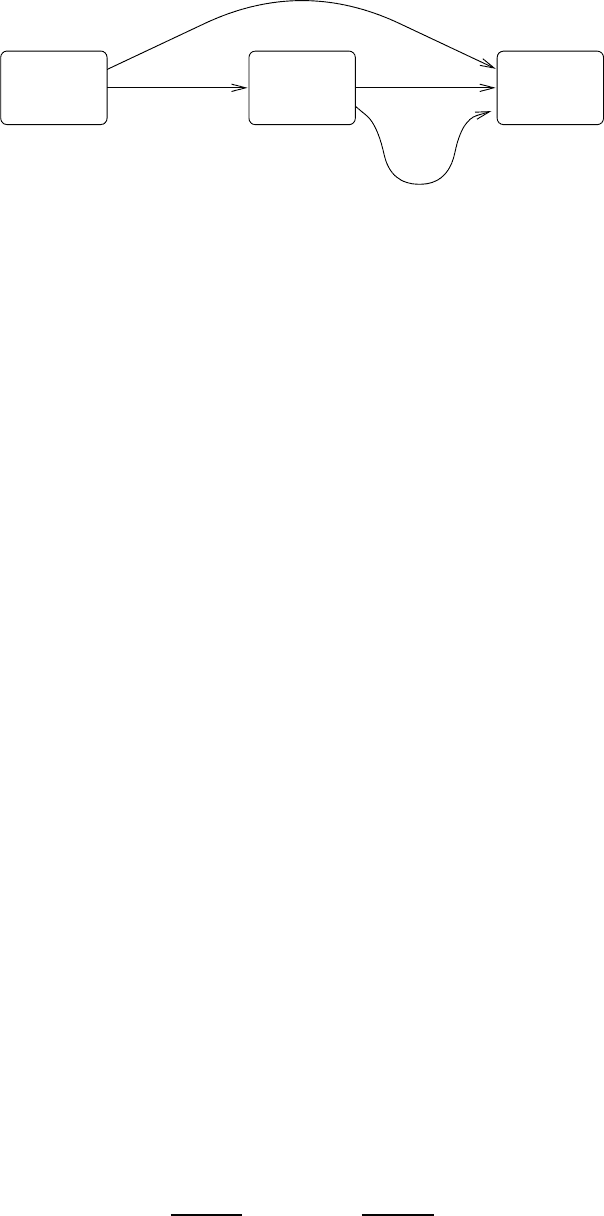
The second proof of Theorem 7.10 consists of showing that the construction employed in

the ﬁrst step, when composed with Theorem 7.8, actually yields the desired end result. This

proof will uncover a connection between hardness ampliﬁcation and coding theory. Our

presentation will thus proceed in three corresponding steps (presented in §7.2.1.1–7.2.1.3,

and schematically depicted in Figure 7.2).

257

CUUS063 main CUUS063 Goldreich 978 0 521 88473 0 March 31, 2008 18:49

THE BRIGHT SIDE OF HARDNESS

worst-case

HARDNESS

average-case

mild

via list decoding (7.2.1.3)

7.2.1.1 7.2.1.2

Yao’s XOR

derandomized

Yao’s XOR (7.2.2)

inapprox.

Figure 7.2: Proofs of hardness ampliﬁcation: Organization.

7.2.1.1. From Worst-Case Hardness to Mild Average-Case Hardness

The transformation of worst-case hardness into average-case hardness (even in a mild

sense) is indeed remarkable. Note that worst-case hardness may be due to a relatively

small number of instances, whereas even mild for ms of average-case hardness refer to

a very large number of possible instances.

In other words, we should transform hard-

ness that may occur on a negligible fraction of the instances into hardness that occurs

on a noticeable fraction of the instances. Intuitively, we should “spread” the hardness

of few instances (of the original problem) over all (or most) instances (of the trans-

formed problem). The counter-positive view is that computing the value of typical in-

stances of the transformed problem should enable solving the original problem on every

instance.

The aforementioned transformation is based on the self-correction paradigm,tobe

reviewed ﬁrst. The paradigm refers to functions g that can be evaluated at any desired

point by using the value of g at a few random points, where each of these points is

uniformly distributed in the function’s domain (but indeed the points are not independently

distributed). The key observation is that if g(x) can be reconstructed based on the value

of g at t such random points, then such a reconstr uction can tolerate a 1/3t fraction of

errors (regarding the values of g). Thus, if we can correctly obtain the value of g on

all but at most a 1/3t fraction of its domain, then we can probabilistically recover the

correct value of g at any point with very high probability. It follows that if no probabilistic

polynomial-time algorithm can correctly compute g in the worst-case sense, then every

probabilistic polynomial-time algorithm must fail to correctly compute g on more than a

1/3t fraction of its domain.

The archetypical example of a self-correctable function is any m-variate polynomial

of individual degree d over a ﬁnite ﬁeld F such that |F| > dm + 1. The value of such a

polynomial at any desired point x can be recovered based on the values of dm + 1 points

(other than x) that reside on a random line that passes through x. Note that each of these

points is uniformly distributed in F

, which is the function’s domain. (For details, see

Exercise 7.11.)

Recall that we are given an arbitrary function f ∈ E that is hard to compute in the worst

case. Needless to say, this function is not necessarily self-correctable (based on relatively

Indeed, worst-case hardness with respect to polynomial-size circuits cannot be due to a polynomial number of

instances, because a polynomial number of instances can be hard-wired into such circuits. Still, for all we know, worst-

case hardness may be due to a small super-polynomial number of instances (e.g., n

log

instances). In contrast, even

mild forms of average-case hardness must be due to an exponential number of instances (i.e., 2

/poly(n) instances).

258

CUUS063 main CUUS063 Goldreich 978 0 521 88473 0 March 31, 2008 18:49

7.2. HARD PROBLEMS IN E

few points), but it can be extended into such a function. Speciﬁcally, we extend f :[N] →

{0, 1} (viewed as f :[N

1/m

]

→{0, 1})toanm-variate polynomial of individual degree

d over a ﬁnite ﬁeld F such that |F| > dm + 1 and ( d + 1)

= N. Intuitively, in terms of

worst-case complexity, the extended function is at least as hard as f , which means that it

is hard (in the worst case). The point is that the extended function is self-correctable and

thus its worst-case hardness implies that it must be at least mildly hard in the average-case.

Details follow.

Construction 7.11 (multivariate extension):

For any function f

: {0, 1}

→

{0, 1}, a ﬁnite ﬁeld F, a set H ⊂ F, and an integer m such that |H |

= 2

and

|F| > (|H |−1)m + 1, we consider the function

: F

→ F deﬁned as the m-

variate polynomial of individual degree |H|−1 that extends f

: H

→{0, 1}.

That is, we identify {0, 1}

with H

, and deﬁne

as the unique m-variate poly-

nomial of individual degree |H |−1 that satisﬁes

(x) = f

(x) for every x ∈ H

where we view {0, 1} as a subset of F.

Note that

can be evaluated at any desired point, by evaluating f

on its entire domain,

and determining the unique m-variate polynomial of individual degree |H |−1 that agrees

with f

on H

(see Exercise 7.12). Thus, for f : {0, 1}

∗

→{0, 1} in E, the corresponding

f (deﬁned by separately extending the restriction of f to each input length) is also in E.

For the sake of preserving various complexity measures, we wish to have |F

|=poly(2

which leads to setting m = n/ log

n (yielding |H |=n and |F|=poly(n)). In particular,

in this case

is deﬁned over strings of length O(n). The mild average-case hardness of

f follows by the foregoing discussion. In fact, we state and prove a more general result.

Theorem 7.12: Suppose that there exists a Boolean function f in E having cir-

cuit complexity that is almost-everywhere greater than S. Then, there exists an

exponential-time computable function

f : {0, 1}

∗

→{0, 1}

∗

such that |

f (x)|≤|x|

and for every family of circuit {C



}



∈N

of size S



) = S(n



/O(1))/poly(n



) it holds

that

Pr[C



) =

f (U



)] > (1/n



)

. Furthermore,

f does not depend on S.

Theorem 7.12 seems to complete the ﬁrst step of the proof of Theorem 7.10, except that

we desire a Boolean function rather than a function that merely does not stretch its input.

The extra step of obtaining a Boolean function that is (poly(n), n

−3

)-inapproximable is

taken in Exercise 7.13.

Essentially, if

f is hard to compute on a noticeable fraction of its

inputs then the Boolean predicate that on input (x, i ) returns the i

bit of

f (x) must be

mildly inapproximable.

Proof Sketch: Given f as in the hypothesis and for every n ∈ N, we consider the

restriction of f to {0, 1}

, denoted f

, and apply Construction 7.11 to it, while

using m = n/ log n, |H |=n and n

< |F|=poly(n). Recall that the resulting

function

maps strings of length n



= log

|=O(n) to strings of length

The algebraic fact underlying this construction is that for any function f : H

→ F there exists a unique m-

variate polynomial

f : F

→ F of individual degree |H |−1 such that for every x ∈ H

it holds that

f (x) = f (x).

This polynomial is called a multivariate polynomial extension of f , and it can be found in poly(|H |

log |F|)-time.

For details, see Exercise 7.12.

A quantitatively stronger bound can be obtained by noting that the proof of Theorem 7.12 actually establishes

an error lower bound of ((log n



)/(n



)

) and that |

f (x)|=O(log |x|).

259

CUUS063 main CUUS063 Goldreich 978 0 521 88473 0 March 31, 2008 18:49

THE BRIGHT SIDE OF HARDNESS

log

|F|=O(log n). Following the foregoing discussion, we shall show that cir-

cuits that approximate

too well yield circuits that compute f

correctly on each

input. Using the hypothesis regarding the size of the latter, we shall derive a lower

bound on the size of the former. The actual (reducibility) argument proceeds as

follows. We ﬁx an arbitrary circuit C



that satisﬁes

Pr[C



) =



)] ≥ 1 − (1/n



)

> 1 − (1/3t), (7.9)

where t

def

= (|H|−1)m + 1 = o(n

) exceeds the total degree of

. Using the self-

correction feature of

, we observe that by making t oracle calls to C



we can

probabilistically recover the value of (

and thus of) f

on each input, with proba-

bility at least 2/3. Using error reduction and (non-uniform) derandomization as in

the proof of Theorem 6.3,

we obtain a circuit of size n

·|C



| that computes f

By the hypothesis n

·|C



| > S(n), and so |C



| > S(n



/O(1))/poly(n



). Recalling

that C



is an arbitrary circuit that satisﬁes Eq. (7.9), the theorem follows.

Digest. The proof of Theorem 7.12 is actually a worst-case to average-case reduction.

That is, the proof consists of a self-correction procedure that allows for the evaluation of f

at any desired n-bit long point, using oracle calls to any circuit that computes

f correctly

on a 1 −(1/n



)

fraction of the n



-bit long inputs. We recall that if f ∈ E then

f ∈ E,

but we do not know how to preserve the complexity of f in case it is in NP. (Various

indications to the difﬁculty of a worst-case to average-case reduction for NP are known;

see, e.g., [43].)

We mention that the ideas underlying the proof of Theorem 7.12 have been applied in

a large variety of settings. For example, we shall see applications of the self-correction

paradigm in §9.3.2.1 and in §9.3.2.2. Furthermore, in §9.3.2.2 we shall reencounter the

very same multivariate extension used in the proof of Theorem 7.12.

7.2.1.2. Yao’s XOR Lemma

Having obtained a mildly inapproximable predicate, we wish to obtain a strongly inapprox-

imable one. The information-theoretic context provides an appealing suggestion: Suppose

that X is a Boolean random variable (representing the mild inapproximability of the afore-

mentioned predicate) that equals 1 with probability ε. Then XORing the outcome of n/ε

independent samples of X yields a bit that equals 1 with probability 0.5 ± exp(−(n)).

It is tempting to think that the same should happen in the computational setting. That is,

if f is hard to approximate correctly with probability exceeding 1 − ε then XORing the

output of f on n/ε non-overlapping parts of the input should yield a predicate that is

hard to approximate correctly with probability that is non-negligibly higher than 1/2. The

latter assertion turns out to be correct, but (even more than in Section 7.1.2) the proof

of the computational phenomenon is considerably more complex than the analysis of the

information-theoretic analogue.

Theorem 7.13 (Yao’s XOR Lemma): There exists a universal constant c > 0 such

that the following holds. If, for some polynomials p

and p

, the Boolean function f is

First, we apply the foregoing probabilistic procedure O(n) times and take a majority vote. This yields a

probabilistic procedure that, on input x ∈{0, 1}

,invokesC



for o(n

) times and computes f

(x ) correctly with

probability greater than 1 − 2

−n

. Finally, we just ﬁx a sequence of random choices that is good for all 2

possible

inputs, and obtain a circuit of size n

·|C



| that computes f

correctly on every n-bit input.

260

CUUS063 main CUUS063 Goldreich 978 0 521 88473 0 March 31, 2008 18:49

7.2. HARD PROBLEMS IN E

, 1/ p

)-inapproximable, then the function F(x

,...,x

t(n)

) =⊕

t(n)

i=1

f (x

), where

t(n) = n · p

(n) and x

,...,x

t(n)

∈{0, 1}

,is p



-inapproximable for p



(t(n) · n) =

(n)

/t(n)

1/c

. Furthermore, the claim also holds if the polynomials p

and p

are

replaced by any integer functions.

Combining Theorem 7.12 (and Exercise 7.13), and Theorem 7.13, we obtain a proof of

Theorem 7.10. (Recall that an alternative proof is presented in §7.2.1.3.)

We note that proving Theorem 7.13 seems more difﬁcult than proving Theorem 7.5 (i.e.,

the ampliﬁcation of one-way functions), due to two issues. Firstly, unlike in Theorem 7.5,

the computational problems are not in PC and thus we cannot efﬁciently recognize

correct solutions to them. Secondly, unlike in Theorem 7.5, solutions to instances of the

transformed problem do not correspond to the concatenation of solutions for the original

instances, but are rather a function of the latter that loses almost all the information

about the latter. The proof of Theorem 7.13 presented next deals with each of these two

difﬁculties separately.

Several different proofs of Theorem 7.13 are known. As just stated, the proof that

we present is conceptually appealing because it deals separately with two unrelated dif-

ﬁculties. Furthermore, this proof beneﬁts most from the material already presented in

Section 7.1. The proof proceeds in two steps:

1. First we prove that the corresponding “direct product” function P(x

,...,x

t(n)

) =

( f (x

),..., f (x

t(n)

)) is difﬁcult to compute in a strong average-case sense.

2. Next we establish the desired result by an application of Theorem 7.8.

Thus, given Theorem 7.8, our main focus is on the ﬁrst step, which is of independent

interest (and is thus generalized from Boolean functions to arbitrary ones).

Theorem 7.14 (the Direct Product Lemma): Let p

and p

be two polynomials,

and suppose that f : {0, 1}

∗

→{0, 1}

∗

is such that for every family of p

-size cir-

cuits, {C

}

n∈N

, and all sufﬁciently large n ∈ N, it holds that Pr[C

) = f (U

)] >

1/ p

(n).LetP(x

,...,x

t(n)

) = ( f (x

),..., f (x

t(n)

)), where x

,...,x

t(n)

∈{0, 1}

and t(n) = n · p

(n). Then, for any ε



: N → (0, 1], setting p



such that p



(t(n) ·

n) = p

(n)/poly(t(n)/ε



(t(n) · n)), it holds that every family of p



-size circuits,



}

m∈N

, satisﬁes Pr[C



) = P(U

)] <ε



(m). Furthermore, the claim also

holds if the polynomials p

and p

are replaced by any integer functions.

In particular, for an adequate constant c > 0, selecting ε



(t(n) · n) = p

(n)

−c

, we obtain



(t(n) · n) = p

(n)

/t(n)

1/c

, and so ε



(m) ≤ 1/ p



(m).

Deriving Theorem 7.13 from Theorem 7.14. Theorem 7.13 follows from Theorem 7.14

by considering the function P



,...,x

t(n)

, r) = b( f (x

) ··· f (x

t(n)

), r), where f is a

Boolean function, r ∈{0, 1}

t(n)

, and b(y, r) is the inner-product modulo 2 of the t(n)-bit

long strings y and r. Note that, for the corresponding P,wehaveP



,...,x

t(n)

, r) ≡

b(P(x

,...,x

t(n)

), r), whereas F(x

,...,x

t(n)

) = P



,...,x

t(n)

, 1

t(n)

). Intuitively, the

inapproximability of P



should follow from the strong average-case hardness of P (via

Theorem 7.8), whereas it should be possible to reduce the approximation of P



to the

approximation of F (and thus derive the desired inapproximability of F). Indeed, this

261

CUUS063 main CUUS063 Goldreich 978 0 521 88473 0 March 31, 2008 18:49

THE BRIGHT SIDE OF HARDNESS

intuition does not fail, but detailing the argument seems a bit cumbersome (and so

we only provide the clues here). Assuming that f is ( p

, 1/ p

)-inapproximable, we

ﬁrst apply Theorem 7.14 (with ε



(t(n) · n) = p

(n)

−c

) and then apply Theorem 7.8 (see

Exercise 7.14), inferring that P



is p



-inapproximable for p



(t(n) · n) =

(n)

(1)

/poly(t(n)). The less obvious part of the argument is reducing the approximation

of P



to the approximation of F. The key observation is that



,...,x

t(n)

, r) = F(z

,...,z

t(n)

) ⊕

i:r

f (z

) (7.10)

where z

= x

if r

= 1 and is an arbitrary n-bit long string otherwise. Now, if somebody

provides us with samples of the distribution (U

, f (U

)), then we can use these samples

in the role of the pairs (z

, f (z

)) for the indices i that satisfy r

= 0. Considering a best

choice of such samples (i.e., one for which we obtain the best approximation of P



), we

obtain a circuit that approximates P



(by using a circuit that approximates F and the said

choices of samples). (The details are left for Exercise 7.17.) Theorem 7.13 follows.

Proving Theorem 7.14. Note that Theorem 7.14 is closely related to Theorem 7.5; see

Exercise 7.20 for details. This suggests employing an analogous proof strategy, that is,

converting circuits that violate the theorem’s conclusion into circuits that violate the

theorem’s hypothesis. We note, however, that things were much simpler in the context of

Theorem 7.5: There we could (efﬁciently) check whether or not a value contained in the

output of the circuit that solves the direct-product problem constitutes a correct answer

for the corresponding instance of the basic problem. Lacking such an ability in the current

context, we shall have to use such values more carefully. Loosely speaking, we shall take a

weighted majority vote among various answers, where the weights reﬂect our conﬁdence

in the correctness of the various answers.

We establish Theorem 7.14 by applying the following lemma that provides quantitative

bounds on the feasibility of computing the direct product of two functions. In this lemma,

}

m∈N

and {Z

}

m∈N

are independent probability ensembles such that Y

, Z

∈{0, 1}

and X

= ( Y

(n)

, Z

n−(n)

) for some function  :N →N. The lemma refers to the suc-

cess probability of computing the direct product function F : {0, 1}

∗

→{0, 1}

∗

deﬁned by

F(yz) = (F

(y), F

(z)), where |y|=(|yz|), when given bounds on the success probabil-

ity of computing F

and F

(separately). Needless to say, these probability bounds refer

to circuits of certain sizes. (The slackness parameter ε represents a deviation from an

idealized result in which the probability of correctly computing F is upper-bounded by

the product of the probabilities of correctly computing F

and F

, where tightening this

slackness (i.e., decreasing ε) comes at the cost of decreasing the size of the circuit for

which the success probability bound holds.) We stress that the lemma is not symmetric with

respect to the two functions: It guarantees a stronger (and in fact lossless) preservation

of circuit sizes for one of the functions (which is arbitrarily chosen to be F

Lemma 7.15 (Direct Product, a quantitative two-argument version): For {Y

},F

, , {X

} and F as in the foregoing, let ρ

(·) be an upper bound

on the success probability of s

(·)-size circuits in computing F

over {Y

}. That is,

for every such circuit family {C

}

Pr[C

)=F

)] ≤ ρ

(m)

262

CUUS063 main CUUS063 Goldreich 978 0 521 88473 0 March 31, 2008 18:49

7.2. HARD PROBLEMS IN E

Likewise, suppose that ρ

(·) is an upper bound on the probability that s

(·)-size

circuits compute F

over {Z

}. Then, for every function ε : N →R, the function ρ

deﬁned as

ρ(n)

def

= ρ

((n)) · ρ

(n − (n)) + ε(n)

is an upper bound on the probability that families of s(·)-size circuits correctly

compute F over {X

}, where

s(n)

def

= min



((n)),

(n − (n))

poly(n/ε(n))



Theorem 7.14 is derived from Lemma 7.15 by using a careful induction, which capitalizes

on the highly quantitative form of Lemma 7.15 and in particular on the fact that no loss is

incurred for one of the two functions that are used. We ﬁrst detail this argument, and next

establish Lemma 7.15 itself.

Deriving Theorem 7.14 from Lemma 7.15. We write P(x

, x

,...,x

t(n)

)as

(t(n))

, x

,...,x

t(n)

), where P

(i)

,...,x

) = ( f (x

),..., f (x

)) and P

(i)

,...,

) ≡ (P

(i−1)

,...,x

i−1

), f (x

)). For any function ε, we shall prove by induction on

i that circuits of size s(n) = p

(n)/poly(t(n)/ε(n)) cannot compute P

(i)

i·n

) with suc-

cess probability greater than (1 −(1/p

(n)))

+ (i − 1) · ε(n), where p

and p

areasin

Theorem 7.14. Thus, no s(n)-size circuit can compute P

(t(n))

t(n)·n

) with success prob-

ability greater than (1 −(1/p

(n))

t(n)

+ (t(n) −1) · ε(n) = exp(−n) +(t(n) − 1) ·ε(n).

Recalling that this is established for any function ε, Theorem 7.14 follows (by us-

ing ε(n) = ε



(t(n) · n)/t(n), and observing that the setting s(n) = p



(t(n) · n) satisﬁes

s(n) = p

(n)/poly(t(n)/ε(n))).

Turning to the induction itself, we ﬁrst note that its basis (i.e., i = 1) is guaranteed by

the theorem’s hypothesis (i.e., the hypothesis of Theorem 7.14 regarding f ). The induction

step (i.e., from i to i + 1) will be proved by using Lemma 7.15 with F

= P

(i)

and F

= f ,

along with the parameter setting ρ

(i)

(i · n) = (1 − (1/ p

(n))

+ (i − 1) · ε(n), s

(i)

(i · n) =

s(n), ρ

(i)

(n) = 1 − (1/ p

(n)) and s

(i)

(n) = poly(n/ε(n)) · s(n) = p

(n). Details follow.

Note that the induction hypothesis (regarding P

(i)

) implies that F

satisﬁes the hypoth-

esis of Lemma 7.15 (wrt size s

(i)

and success rate ρ

(i)

), whereas the theorem’s hypothesis

regarding f implies that F

satisﬁes the hypothesis of Lemma 7.15 (wrt size s

(i)

and suc-

cess rate ρ

(i)

). Thus, F = P

(i+1)

satisﬁes the lemma’s conclusion with respect to circuits of

size min(s

(i)

(i · n), s

(i)

(n)/poly(n/ε(n))) = s(n) and success rate ρ

(i)

(i · n) ·ρ

(i)

(n) + ε(n)

which is upper-bounded by (1 − (1/p

(n)))

i+1

+i · ε(n). This completes the induction

step.

We stress the fact that we used induction for a non-constant number of steps, and that

this was enabled by the highly quantitative form of the inductive claim and the small loss

incurred by the inductive step. Speciﬁcally, the size bound did not decrease during the

induction (although we could afford a small additive loss in each step, but not a constant

factor loss).

Likewise, the success rate suffered an additive increase of ε(n) in each

Note that if we had s(n) = min{s

((n)), s

(n − (n))}/2 (in Lemma 7.15) then the foregoing argument would

yield that P

(i+1)

is hard for circuits of size s

(i+1)

such that s

(i+1)

((i + 1) · n) = min{s

(i)

(i · n), s

(n)}/2, which

would yield a meaningless result for P = P

(t(n))

(since s

(t(n))

(t(n) · n) = min{p

(n), p

(n)}/2

t(n)

,wheret (n)  n

and p

(n) < 2

263

CUUS063 main CUUS063 Goldreich 978 0 521 88473 0 March 31, 2008 18:49

THE BRIGHT SIDE OF HARDNESS

step, which was accommodated by the inductive claim. Thus, assuming the correctness

of Lemma 7.15, we have established Theorem 7.14.

Proof of Lemma 7.15: Proceeding (as usual) by the contra-positive, we consider

a family of s(·)-size circuits {C

}

n∈N

that violates the lemma’s conclusion; that is,

Pr[C

) = F(X

)] >ρ(n). We will show how to use such circuits in order to

obtain either circuits that violate the lemma’s hypothesis regarding F

or circuits

that violate the lemma’s hypothesis regarding F

. Toward this end, it is instructive

to write the success probability of C

in a conditional form, while denoting the i

output of C

(x)byC

(x)

(i.e., C

(x) = (C

(x)

, C

(x)

)):

Pr[C

(n)

, Z

n−(n)

)=F(Y

(n)

, Z

n−(n)

)]

Pr[C

(n)

, Z

n−(n)

)

(n)

)]

Pr[C

(n)

, Z

n−(n)

)

n−(n)

) |C

(n)

, Z

n−(n)

)

(n)

)].

The basic idea is that if the ﬁrst factor is greater than ρ

((n)) then we immediately

derive a circuit (i.e., C



(y) = C

(y, Z

n−(n)

)

) contradicting the lemma’s hypothesis

regarding F

, whereas if the second factor is signiﬁcantly greater than ρ

(n − (n))

then we can obtain a circuit contradicting the lemma’s hypothesis regarding F

. The

treatment of the latter case is indeed not obvious. The idea is that a sufﬁciently

large sample of (Y

(n)

, F

(n)

)), which may be hard-wired into the circuit, allows

for using the conditional probability space (in such a circuit) toward an attempt

to approximate F

. That is, on input z, we select uniformly a string y satisfying

(y, z)

= F

(y) (from the aforementioned sample), and output C

(y, z)

.Fora

ﬁxed z, sampling of the conditional space (i.e., y’s satisfying C

(y, z)

= F

(y)) is

possible provided that

Pr[C

(n)

, z)

(n)

)] holds with noticeable probability.

The last caveat motivates a separate treatment of z’s having a noticeable value of

Pr[C

(n)

, z)

(n)

)] and of the rest of z’s (which are essentially ignored).

Details follow.

Let us ﬁrst simplify the notations by ﬁxing a generic n and using the abbreviations

C = C

, ε = ε(n),  = (n), Y = Y



, and Z = Y

n−

. We call z good if Pr[C(Y, z)

(Y )] ≥ ε/2 and let G be the set of good z’s. Next, rather than considering the event

C(Y, Z ) =F(Y, Z), we consider the combined event C(Y, Z)=F(Y, Z ) ∧ Z ∈G,

which occurs with almost the same probability (up to an additive error term of ε/2).

This is the case because, for any z ∈ G, it holds that

Pr[C(Y, z) =F(Y, z)] ≤ Pr[C(Y, z)

(Y )] <ε/2

and thus z’s that are not good do not contribute much to

Pr[C(Y, Z)=F(Y, Z)]; that

is,

Pr[C(Y, Z)=F(Y, Z) ∧ Z ∈G] is lower-bounded by Pr[C(Y, Z)=F(Y , Z )] −

ε/2. Using

Pr[C(Y, z)=F(Y, z)] >ρ(n) = ρ

() ·ρ

(n − ) + ε,wehave

Pr[C(Y, Z)=F(Y, Z) ∧ Z ∈G] >ρ

() ·ρ

(n − ) +

(7.11)

We proceed according to the foregoing outline, ﬁrst showing that if

Pr[C(Y, Z)

(Y )] >ρ

() then we immediately derive circuits violating the hypothesis con-

cerning F

. Actually, we prove something stronger (which we will need for the other

case).

Claim 7.15.1: For every z, it holds that Pr[C(Y, z)

(Y )] ≤ ρ

().

264