Goldreich O. Computational Complexity. A Conceptual Perspective

Подождите немного. Документ загружается.

CUUS063 main CUUS063 Goldreich 978 0 521 88473 0 March 31, 2008 18:49

8.2. GENERAL-PURPOSE PSEUDORANDOM GENERATORS

Pr[D(U

(k(n))

)=1] − Pr[D(G(U

k(n)

))=1] is lower-bounded by the expectation of

Eq. (8.5), which equals

E[|

A,T

(F(1

))|] −E[η(F(1

))]. Combining the hypothesis

that

E[|

A,T

(F(1

))|] >ε(n) and the fact that max

x∈{0,1}

{η(x)}≤ε(n)/2, we infer

that

Pr[D(U

(k(n))

)=1] − Pr[D(G(U

k(n)

))=1] >ε(n)/2. Recalling that D runs in

time poly(n/ε(n)), this contradicts the pseudorandomness of G. The proposition

follows.

Conclusion. Although the foregoing refers to standard probabilistic polynomial-time

algorithms, a similar construction and analysis applies to any efﬁcient randomized process

(i.e., any efﬁcient multi-party computation). Any such process preserves its behavior when

replacing its perfect source of randomness (postulated in its analysis) by a pseudorandom

sequence (which may be used in the implementation). Thus, given a pseudorandom

generator with a large stretch function, one can considerably reduce the randomness

complexity of any efﬁcient application.

8.2.3. Computational Indistinguishability

In this section we spell out (and study) the deﬁnition of computational indistinguishability

that underlies Deﬁnition 8.1.

8.2.3.1. The General Formulation

The (general formulation of the) deﬁnition of computational indistinguishability refers

to arbitrary probability ensembles. Here, a

probability ensemble is an inﬁnite sequence

of random variables {Z

}

n∈N

such that each Z

ranges over strings of length that is

polynomially related to n (i.e., there exists a polynomial p such that for every n it holds

that |Z

|≤p(n) and p(|Z

|) ≥ n). We say that {X

}

n∈N

and {Y

}

n∈N

are computationally

indistinguishable

if for every feasible algorithm A the difference d

(n)

def

=|Pr[A(X

) =

1] −

Pr[A(Y

) = 1]| is a negligible function in n. That is:

Deﬁnition 8.4 (computational indistinguishability): The probability ensembles

}

n∈N

and {Y

}

n∈N

are computationally indistinguishable if for every probabilis-

tic polynomial-time algorithm D, every positive polynomial p, and all sufﬁciently

large n,

Pr[D(X

)=1] −Pr[D(Y

)=1]| <

p(n)

(8.6)

where the probabilities are taken over the relevant distribution (i.e., either X

) and over the internal coin tosses of algorithm D. The l.h.s. of Eq. (8.6), when

viewed as a function of n, is often called the

distinguishing gap of D, where {X

}

n∈N

and {Y

}

n∈N

are understood from the context.

We can think of D as representing somebody who wishes to distinguish two distributions

(based on a given sample drawn from one of the distributions), and think of the output “1”

as representing D’s verdict that the sample was drawn according to the ﬁrst distribution.

Saying that the two distributions are computationally indistinguishable means that if D

is a feasible procedure then its verdict is not really meaningful (because the verdict is

almost as often 1 when the sample is drawn from the ﬁrst distribution as when the sample

295

CUUS063 main CUUS063 Goldreich 978 0 521 88473 0 March 31, 2008 18:49

PSEUDORANDOM GENERATORS

is drawn from the second distribution). We comment that the absolute value in Eq. (8.6)

can be omitted without affecting the deﬁnition (see Exercise 8.3), and we will often do so

without warning.

In Deﬁnition 8.1, we required that the probability ensembles {G(U

)}

k∈N

and {U

(k)

}

k∈N

be computationally indistinguishable. Indeed, an important special case of Deﬁnition 8.4

is when one ensemble is uniform, and in such a case we call the other ensemble

pseudo-

random

8.2.3.2. Relation to Statistical Closeness

Two probability ensembles, {X

}

n∈N

and {Y

}

n∈N

, are said to be statistically close (or sta-

tistically indistinguishable) if for ever y positive polynomial p and all sufﬁcient large n the

variation distance between X

and Y

(i.e.,



|Pr[X

= z] − Pr[Y

= z]|) is bounded

above by 1/ p(n). Clearly, any two probability ensembles that are statistically close are

computationally indistinguishable. Needless to say, this is a trivial case of computational

indistinguishability, which is due to information-theoretic reasons. In contrast, we shall be

interested in non-trivial cases (of computational indistinguishability), which correspond

to probability ensembles that are statistically far apart.

Indeed, as noted in Section 8.1, there exist probability ensembles that are statisti-

cally far apart and yet are computationally indistinguishable (see Exercise 8.1). However,

at least one of the probability ensembles in Exercise 8.1 is not polynomial-time con-

structible.

We shall be much more interested in non-trivial cases of computational indis-

tinguishability in which both ensembles are polynomial-time constructible. An important

example is provided by the deﬁnition of pseudorandom generators (see Exercise 8.7). As

we shall see (in Theorem 8.11), the existence of one-way functions implies the existence

of pseudorandom generators, which in turn implies the existence of polynomial-time

constructible probability ensembles that are statistically f ar apart and yet are computa-

tionally indistinguishable. We mention that this sufﬁcient condition is also necessary (see

Exercise 8.9).

8.2.3.3. Indistinguishability by Multiple Samples

The deﬁnition of computational indistinguishability (i.e., Deﬁnition 8.4) refers to distin-

guishers that obtain a single sample from one of the two relevant probability ensembles

(i.e., {X

}

n∈N

and {Y

}

n∈N

). A very natural generalization of Deﬁnition 8.4 refers to

distinguishers that obtain several independent samples from such an ensemble.

Deﬁnition 8.5 (indistinguishability by multiple samples): Let s : N →N be poly-

nomially bounded. Two probability ensembles, {X

}

n∈N

and {Y

}

n∈N

,are

computationally indistinguishable by s(·) samples if for every probabilistic

polynomial-time algorithm D, every positive polynomial p(·), and all sufﬁciently

large n’s





(1)

,...,X

(s(n))



= 1

− Pr



(1)

,...,Y

(s(n))



= 1



p(n)

where X

(1)

through X

(s(n))

and Y

(1)

through Y

(s(n))

are independent random variables

such that each X

(i)

is identical to X

and each Y

(i)

is identical to Y

We say t hat {Z

}

n∈N

is polynomial-time constructible if there exists a polynomial-time algorithm S such that

S(1

)andZ

are identically distributed.

296

CUUS063 main CUUS063 Goldreich 978 0 521 88473 0 March 31, 2008 18:49

8.2. GENERAL-PURPOSE PSEUDORANDOM GENERATORS

It turns out that in the most interesting cases, computational indistinguishability by a

single sample implies computational indistinguishability by any polynomial number of

samples. One such case is the case of polynomial-time constructible ensembles. We say

that the ensemble {Z

}

n∈N

is polynomial-time constructible if there exists a polynomial-

time algorithm S such that S(1

) and Z

are identically distributed.

Proposition 8.6: Suppose that X

def

={X

}

n∈N

and Y

def

={Y

}

n∈N

are both

polynomial-time constructible, and s be a polynomial. Then, X and Y are computa-

tionally indistinguishable by a single sample if and only if they are computationally

indistinguishable by s(·) samples.

Clearly, for every polynomial s, computational indistinguishability by s(·) samples implies

computational indistinguishability by a single sample (see Exercise 8.5). We now prove

that, for efﬁciently constructible ensembles, indistinguishability by a single sample implies

indistinguishability by multiple samples.

The proof provides a simple demonstration of

a central proof technique, known as the hybrid technique.

Proof Sketch:

Again, the proof uses the counter-positive, which in such settings is

called a reducibility argument (see Section 7.1.2 onward). Speciﬁcally, we show that

the existence of an efﬁcient algorithm that distinguishes the ensembles X and Y using

several samples implies the existence of an efﬁcient algorithm that distinguishes the

ensembles X and Y using a single sample. The implication is proven using the

following argument, which will be later called a “hybrid argument”.

To prove that a sequence of s(n) samples drawn independently from X

is in-

distinguishable from a sequence of s(n) samples drawn independently from Y

we consider hybrid sequences such that the i

hybrid consists of i samples of

followed by s(n) − i samples of Y

. The “homogeneous” sequences (which we

wish to prove to be computational indistinguishable) are the extreme hybrids (i.e.,

the ﬁrst and last hybrids). The key observation is that distinguishing the extreme

hybrids (toward the contradiction hypothesis) implies distinguishing neighboring

hybrids, which in turn yields a procedure for distinguishing single samples of the

two original distributions (contradicting the hypothesis that these two distributions

are indistinguishable by a single sample). Details follow.

Suppose, toward the contradiction, that D distinguishes s(n) samples of X

from

s(n) samples of Y

, with a distinguishing gap of δ(n). Denoting the i

hybrid by H

(i.e., H

= (X

(1)

,...,X

(i)

, Y

(i+1)

,...,Y

(s(n))

)), this means that D distinguishes the

extreme hybrids (i.e., H

and H

s(n)

) with gap δ(n). It follows that D distinguishes

a random pair of neighboring hybrids (i.e., D distinguishes H

from H

i+1

,fora

randomly selected i ) with gap at least δ(n)/s(n): the reason being that

i∈{0,...,s(n)−1}





= 1

− Pr



i+1



= 1

s(n)

s(n)−1



i=0







= 1

− Pr



i+1



= 1



(8.7)

s(n)







= 1

− Pr



s(n)



= 1



δ(n)

s(n)

The requirement that both ensembles are polynomial-time constructible is essential; see Exercise 8.10.

For more details see [91, Sec. 3.2.3].

297

CUUS063 main CUUS063 Goldreich 978 0 521 88473 0 March 31, 2008 18:49

PSEUDORANDOM GENERATORS

The key step in the argument is transforming the distinguishability of neighboring

hybrids into distinguishability of single samples of the original ensembles (thus

deriving a contradiction). Indeed, using D, we obtain a distinguisher D



of single

samples: Given a single sample, algorithm D



selects i ∈{0,...,s(n) − 1} at ran-

dom, generates i samples from the ﬁrst distribution and s(n) −i −1 samples from

the second distribution, invokes D with the s(n)-samples sequence obtained when

placing the input sample in location i + 1, and answers whatever D does. That is,

on input z and when selecting the index i, algorithm D



invokes D on a sample

from the distribution (X

(1)

,...,X

(i)

, z, Y

(i+2)

,...,Y

(s(n))

). Thus, the construction

of D



relies on the hypothesis that both probability ensembles are polynomial-time

constructible. The analysis of D



is based on the following two facts:

1. When invoked on an input that is distributed according to X

and selecting

the index i ∈{0,...,s(n) − 1}, algorithm D



behaves like D(H

i+1

), because

(1)

,...,X

(i)

, X

, Y

(i+2)

,...,Y

(s(n))

) ≡ H

i+1

2. When invoked on an input that is distributed according to Y

and selecting

the index i ∈{0,...,s(n) − 1}, algorithm D



behaves like D(H

), because

(1)

,...,X

(i)

, Y

(i+2)

,...,Y

(s(n))

) ≡ H

Thus, the distinguishing gap of D



(between Y

and X

) is captured by Eq. (8.7),

and the claim follows (because assuming toward the contradiction that the propo-

sition’s conclusion does not hold leads to a contradiction of the proposition’s

hypothesis).

The hybrid technique – a digest. The hybrid technique constitutes a special type of

a “reducibility argument” in which the computational indistinguishability of complex

ensembles is proved using the computational indistinguishability of basic ensembles. The

actual reduction is in the other direction: Efﬁciently distinguishing the basic ensembles is

reduced to efﬁciently distinguishing the complex ensembles, and hybrid distributions are

used in the reduction in an essential way. The following three properties of the construction

of the hybrids play an important role in the argument:

1. The complex ensembles collide with the extreme hybrids. This property is essential

because our aim is proving something that relates to the complex ensembles (i.e.,

their indistinguishability), while the argument itself refers to the extreme hybrids.

In the proof of Proposition 8.6 the extreme hybrids (i.e., H

s(n)

and H

) collide with

the complex ensembles that represent s(n)-ary sequences of samples of one of the

basic ensembles.

2. The basic ensembles are efﬁciently mapped to neighboring hybrids. This property is

essential because our starting hypothesis relates to the basic ensembles (i.e., their in-

distinguishability), while the argument itself refers directly to the neighboring hybrids.

Thus, we need to translate our knowledge (i.e., computational indistinguishability)

of the basic ensembles to knowledge (i.e., computational indistinguishability) of any

pair of neighboring hybrids. Typically, this is done by efﬁciently transforming strings

in the range of a basic distribution into strings in the range of a hybrid such that the

transformation maps the ﬁrst basic distribution to one hybrid and the second basic

distribution to the neighboring hybrid.

298

CUUS063 main CUUS063 Goldreich 978 0 521 88473 0 March 31, 2008 18:49

8.2. GENERAL-PURPOSE PSEUDORANDOM GENERATORS

In the proof of Proposition 8.6 the basic ensembles (i.e., X

and Y

) were efﬁciently

transformed into neighboring hybrids (i.e., H

i+1

and H

, respectively). Recall that,

in this case, the efﬁciency of this transformation relied on the hypothesis that both

the basic ensembles are polynomial-time constructible.

3. The number of hybrids is small (i.e., polynomial). This property is essential in or-

der to deduce the computational indistinguishability of extreme hybrids from the

computational indistinguishability of each pair of neighboring hybrids. Typically, the

“distinguishability gap” established in the argument loses a factor that is proportional

to the number of hybrids. This is due to the fact that the gap between the extreme

hybrids is upper-bounded by the sum of the gaps between neighboring hybrids.

In the proof of Proposition 8.6 the number of hybrids equals s(n) and the aforemen-

tioned loss is reﬂected in Eq. (8.7).

We remark that in the course of a hybrid argument, a distinguishing algorithm referring

to the complex ensembles is being analyzed and even invoked on arbitrary hybrids. The

reader may be annoyed by the fact that the algorithm “was not designed to work on such

hybrids” (but rather only on the extreme hybrids). However, an algorithm is an algorithm:

Once it exists we can invoke it on inputs of our choice, and analyze its performance on

arbitrary input distributions.

8.2.4. Amplifying the Stretch Function

Recall that the deﬁnition of pseudorandom generators (i.e., Deﬁnition 8.1) makes a min-

imal requirement regarding their stretch; that is, it is only required that the length of

the output of such generators be longer than their input. Needless to say, we seek pseu-

dorandom generators with a much more signiﬁcant stretch, ﬁrstly because the stretch

determines the saving in randomness obtained via Constr uction 8.2. It turns out (see Con-

struction 8.7) that pseudorandom generators of any stretch function (and in particular of

minimal stretch 

(k)

def

= k + 1) can be easily converted into pseudorandom generators of

any desired (polynomially bounded) stretch function, . (On the other hand, since pseudo-

random generators are required (in Deﬁnition 8.1) to run in polynomial time, their stretch

must be polynomially bounded.)

Construction 8.7: Let G

be a pseudorandom generator with stretch func-

tion 

(k) = k + 1, and  be any polynomially bounded stretch function that is

polynomial-time computable. Let

G(s)

def

= σ

···σ

(|s|)

(8.8)

where x

= s and x

= G

i−1

),fori= 1,...,(|s|). (That is, σ

is the last bit

of G

i−1

) and x

is the |s|-bit long preﬁx of G

i−1

).)

Needless to say, G is polynomial-time computable and has stretch . An alternative

construction is considered in Exercise 8.11.

Proposition 8.8: Let G

and G be as in Construction 8.7. Then G constitutes a

pseudorandom generator.

Proof Sketch:

The proposition is proven using the hybrid technique, presented

and discussed in Section 8.2.3. Here (for i = 0,...,(k)), we consider the hybrid

For more details, see [91, Sec. 3.3.3].

299

CUUS063 main CUUS063 Goldreich 978 0 521 88473 0 March 31, 2008 18:49

PSEUDORANDOM GENERATORS

i+1

. . .

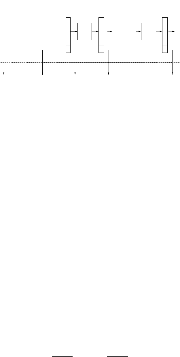
σσ

1 i-1

. . .

i+1

Figure 8.2: Analysis of stretch ampliﬁcation – the i

hybrid.

distributions H

, depicted in Figure 8.2 and deﬁned by

def

= U

(1)

· g

(k)−i



(2)



where · denotes the concatenation of strings, g

(x) denotes the j-bit long preﬁx

of G(x), and U

(1)

and U

(2)

are independent uniform distributions (over {0, 1}

and

{0, 1}

, respectively). The extreme hybrids (i.e., H

and H

) correspond to G(U

)

and U

(k)

, whereas distinguishability of neighboring hybrids can be worked into

distinguishability of G

) and U

k+1

. Details follow.

We shall focus on proving the indistinguishability of neighboring hybrids.

Sup-

pose, toward the contradiction, that algorithm D distinguishes H

from H

i+1

We ﬁrst take a closer look at these hybrids. Note that, for j ≥ 1, it holds that

(s) ≡ (σ, g

j−1

(x)), where xσ = G

(s). Denoting the ﬁrst |x|−1 bits of x by F(x)

and the last bit of x by L(x), we may write g

(s) ≡ (L(G

(s)), g

j−1

(F(G

(s)))) and

(1)

, U

(2)

) ≡ (L(U

k+1

), F(U

k+1

)). It follows that

= U

(1)

· g

(k)−i



(2)



≡



(1)

, L



(2)



, g

((k)−i)−1



(2)



i+1

= U



)

i+1

· g

(k)−i−1



(2)



≡



(1)

, L





)

k+1



, g

((k)−i)−1



F(U



)

k+1



Now, combining the generation of U

(1)

and the evaluation of g

(k)−i−1

with the dis-

tinguisher D, we distinguish the distribution (F(G

(2)

)), L(G

(2)

))) ≡ G

)

from the distrib ution (F(U



)

k+1

), L(U



)

k+1

)) ≡ U

k+1

, in contradiction to the pseudoran-

domness of G

. Speciﬁcally, on input x ∈{0, 1}

k+1

, we uniformly select r ∈{0, 1}

and output D(r · L(x) · g

(k)−i−1

(F(x))). The analysis of the resulting distinguisher

is based on the following two facts:

As usual (when the hybrid technique is used), the distinguishability of the extreme hybrids (which collide with

G(U

)andU

(k)

, respectively) implies the distinguishability of a random pair of neighboring hybrids. Thus, the

following analysis will be applied to a random i (in {0,...,k − 1}), and the full analysis will refer to an expression

analogous to Eq. (8.7).

300

CUUS063 main CUUS063 Goldreich 978 0 521 88473 0 March 31, 2008 18:49

8.2. GENERAL-PURPOSE PSEUDORANDOM GENERATORS

1. When given an input that is distributed according to G

), we invoke algorithm

D on input (U



, L(G

)), g

(k)−i−1

(F(G

)))) ≡ H

2. When given an input that is distributed according to U

k+1

, we invoke algorithm

D on input (U



, L(U

k+1

), g

(k)−i−1

(F(U

k+1

))) ≡ H

i+1

Thus, the probability that we output 1 on input G

) (resp., U

k+1

) equals

Pr[D(H

) = 1] (resp., Pr[D(H

i+1

) = 1]). Hence, the distinguishability of neigh-

boring hybrids implies the distinguishability of G

) and U

k+1

Conclusion. In view of the foregoing, when talking about the mere existence of pseu-

dorandom generators, in the sense of Deﬁnition 8.1, we may ignore the speciﬁc stretch

function.

8.2.5. Constructions

The constructions surveyed in this section “transform” computational difﬁculty, in

the form of one-way functions, into generators of pseudorandomness. Recall that a

polynomial-time computable function is called

one-way if any efﬁcient algorithm can

invert it only with negligible success probability (see Deﬁnition 7.1 and Section 7.1 for

further discussion). We will actually use hard-core predicates of such functions, and refer

the reader to their treatment in Section 7.1.3. Loosely speaking, a polynomial-time com-

putable predicate b is called a

hard-core of a function f if any efﬁcient algorithm, given

f (x), can guess b(x) with success probability that is only negligibly higher than half.

Recall that (by Theorem 7.7), for any one-way function f , the inner-product mod 2 of x

and r is a hard-core of f



(x, r ) = ( f (x), r ).

8.2.5.1. A Simple Construction

Intuitively, the deﬁnition of a hard-core predicate implies a potentially interesting case

of computational indistinguishability. Speciﬁcally, as will be shown implicitly in Propo-

sition 8.9 and explicitly in Exercise 8.8,ifb is a hard-core of the function f , then

the ensemble {f (U

) ·b(U

)}

n∈N

is computationally indistinguishable from the ensemble

{f (U

) ·U



}

n∈N

. Furthermore, if f is 1-1 then the foregoing ensembles are statistically

far apart, and thus constitute a non-trivial case of computational indistinguishability. If f

is also polynomial-time computable and length-preserving, then this yields a construction

of a pseudorandom generator.

Proposition 8.9 (A simple construction of pseudorandom generators): Let b be a

hard-core predicate of a polynomial-time computable 1-1 and length-preserving

function f . Then, G(s)

def

= f (s) · b(s) is a pseudorandom generator.

Proof Sketch:

Considering a uniformly distributed s ∈{0, 1}

, we ﬁrst note that

the n-bit long preﬁx of G(s) is uniformly distributed in {0, 1}

, because f induces

a permutation on the set {0, 1}

. Hence, the proof boils down to showing that

distinguishing f (s) · b(s) from f (s) · σ , where σ is a random bit, yields contradiction

to the hypothesis that b is a hard-core of f (i.e., that b(s)isunpredictable from f (s)).

Intuitively, the reason is that such a hypothetical distinguisher also distinguishes

For more details, see [91, Sec. 3.3.4].

301

CUUS063 main CUUS063 Goldreich 978 0 521 88473 0 March 31, 2008 18:49

PSEUDORANDOM GENERATORS

f (s) · b(s) from f (s) · b(s), where σ = 1 −σ , whereas distinguishing f (s) · b(s)

from f (s) ·

b(s) yields an algorithm for predicting b(s) based on f (s). Details follow.

We start with any potential distinguisher D, and let

δ(k)

def

= Pr[D(G(U

)) = 1] − Pr[D(U

k+1

) = 1].

We may assume, without loss of generality, that δ(k) is non-negative (for inﬁnitely

many k’s). Observing that G(U

) = f (U

) ·b(U

) and that U

k+1

is distributed

identically to a random variable that equals f (U

)b(U

) with probability 1/2 and

f (U

)b(U

) otherwise, we have

Pr[D( f (U

)b(U

)) = 1] − Pr[D( f (U

)b(U

)) = 1] = 2δ(k).

The key observation is that D effectively distinguishes (with gap 2δ(k)) the case that

the last bit is b(U

) from the case that the last bit is b(U

). This distinguishing ability

can be transformed to predicting the value of b(U

), when given the value f (U

Indeed, consider an algorithm A that, on input y, uniformly selects σ ∈{0, 1},

invokes D(yσ ), and outputs σ if D(yσ ) = 1 and

σ otherwise. Then

Pr[A( f (U

)) = b(U

)]

Pr[D( f (U

) ·σ ) = 1 ∧ σ = b(U

)] + Pr[D( f (U

) ·σ ) = 0 ∧ σ = b(U

)]



Pr[D( f (U

) ·b(U

)) = 1] +



1 − Pr[D( f (U

) ·b(U

)) = 1]



which equals (1 + 2δ(k))/2. This contradicts the hypothesis that b is a hard-core of

f , and the proposition follows.

Combining Theorem 7.7, Proposition 8.9, and Construction 8.7, we obtain the following

corollary.

Theorem 8.10 (A sufﬁcient condition for the existence of pseudorandom genera-

tors): If there exists 1-1 and length-preserving one-way function then, for every

polynomially bounded stretch function , there exists a pseudorandom generator of

stretch .

Digest. The main part of the proof of Proposition 8.9 is showing that the (next bit)

unpredictability of G(U

) implies the pseudorandomness of G(U

). The fact that (next

bit) unpredictability and pseudorandomness are equivalent, in general, is proven explicitly

in the alternative proof of Theorem 8.10 provided next.

8.2.5.2. An Alternative Presentation

Let us take a closer look at the pseudorandom generators obtained by combining Con-

struction 8.7 and Proposition 8.9. For a stretch function :N →N, a 1-1 one-way function

f with a hard-core b, we obtain

G(s)

def

= σ

···σ

(|s|)

, (8.9)

where x

= s and x

= f (x

i−1

)b(x

i−1

)fori = 1,...,(|s|). Denoting by f

(x) the

value of f iterated i times on x (i.e., f

(x) = f

i−1

( f (x)) and f

(x) = x), we rewrite

Eq. (8.9) as follows

G(s)

def

= b(s) ·b( f (s)) ···b( f

(|s|)−1

(s)) . (8.10)

302

CUUS063 main CUUS063 Goldreich 978 0 521 88473 0 March 31, 2008 18:49

8.2. GENERAL-PURPOSE PSEUDORANDOM GENERATORS

The pseudorandomness of G is established in two steps, using the notion of (next

bit) unpredictability. An ensemble {Z

}

k∈N

is called unpredictable if any probabilistic

polynomial-time machine obtaining a (random)

preﬁx of Z

fails to predict the next

bit of Z

with probability non-negligibly higher than 1/2. Speciﬁcally, we establish the

following two results.

1. A general result asserting that an ensemble is pseudorandom if and only if it is

unpredictable. Recall that an ensemble is

pseudorandom if it is computationally

indistinguishable from a uniform distribution (over bit strings of adequate length).

Clearly, pseudorandomness implies polynomial-time unpredictability, but here we

actually need the other direction, which is less obvious. Still, using a hybrid argument,

one can show that (next-bit) unpredictability implies indistinguishability from the

uniform ensemble. For details, see Exercise 8.12.

2. A speciﬁc result asserting that the ensemble {G(U

)}

k∈N

is unpredictable from right

to left. Equivalently, G



) is polynomial-time unpredictable (from left to right (as

usual)), where G



(s) = b( f

(|s|)−1

(s)) ···b( f (s)) · b(s) is the reverse of G(s).

Using the fact that f induces a permutation over {0, 1}

, observe that the ( j + 1)-

bit long preﬁx of G



) is distributed identically to b( f

)) ···b( f (U

)) ·b(U

Thus, an algorithm that predicts the j + 1

bit of G



) based on the j-bit long

preﬁx of G



) yields an algorithm that guesses b(U

) based on f (U

). For details,

see Exercise 8.14.

Needless to say, G is a pseudorandom generator if and only if G



is a pseudorandom

generator (see Exercise 8.13). We mention that Eq. (8.10) is often referred to as the

Blum-Micali Construction.

8.2.5.3. A General Condition for the Existence of Pseudorandom Generators

Recall that given any one-way 1-1 length-preserving function, we can easily construct a

pseudorandom generator. Actually, the 1-1 (and length-preserving) requirement may be

dropped, but the currently known construction – for the general case – is quite complex.

Theorem 8.11 (On the existence of pseudorandom generators): Pseudorandom

generators exist if and only if one-way functions exist.

To show that the existence of pseudorandom generators implies the existence of one-

way functions, consider a pseudorandom generator G with stretch function (k) = 2k.

For x, y ∈{0, 1}

, deﬁne f (x, y)

def

= G(x), and so f is polynomial-time computable (and

length-preserving). It must be that f is one-way, or else one can distinguish G(U

) from

by trying to inver t and checking the result: Inverting f on the distribution f (U

)

corresponds to operating on the distrib ution G(U

), whereas the probability that U

has

inverse under f is negligible.

The interesting direction of the proof of Theorem 8.11 is the construction of pseudoran-

dom generators based on any one-way function. Since the known proof is quite complex,

For simplicity, we deﬁne unpredictability as referring to preﬁxes of a random length (distributed uniformly in

{0,...,|Z

|−1}). A more general deﬁnition allows the predictor to determine the length of the preﬁx that it reads

on the ﬂy. This seemingly stronger notion of unpredictability is actually equivalent to the one we use, because both

notions are equivalent to pseudorandomness.

Given the popularity of the term, we deviate from our convention of not specifying credits in the main text.

Indeed, this construction originates in [41].

303

CUUS063 main CUUS063 Goldreich 978 0 521 88473 0 March 31, 2008 18:49

PSEUDORANDOM GENERATORS

we only provide a very rough overview of some of the ideas involved. We mention that

these ideas make extensive use of adequate hashing functions (e.g., pairwise independent

hashing functions; see Appendix D.2).

We ﬁrst note that, in general (when f may not be 1-1), the ensemble f (U

) may not be

pseudorandom, and so Construction 8.9 (i.e., G(s) = f (s)b(s), where b is a hard-core of f )

cannot be used directly. One idea underlying the known construction is hashing f (U

)toan

almost uniform string of length related to its entropy, using adequate hashing functions.

But “hashing f (U

) down to length comparable to the entropy” means shrinking the

length of the output to, say, k



< k. This foils the entire point of stretching the k-bit seed.

Thus, a second idea underlying the construction is compensating for the loss of k − k



bits by extracting these many bits from the seed U

itself. This is done by hashing U

and the point is that the (k − k



)-bit long hash value does not make the inverting task any

easier. Implementing these ideas turns out to be more difﬁcult than it seems, and indeed

an alternative construction would be most appreciated.

8.2.6. Non-uniformly Strong Pseudorandom Generators

Recall that we said that truly random sequences can be replaced by pseudorandom se-

quences without affecting any efﬁcient computation that uses these sequences. The spe-

ciﬁc formulation of this asser tion, presented in Proposition 8.3, refers to randomized

algorithms that take a “primary input” and use a secondary “random-input” in their com-

putation. Proposition 8.3 asserts that it is infeasible to ﬁnd a primary input for which

the replacement of a truly random secondary input by a pseudorandom one affects the

ﬁnal output of the algorithm in a noticeable way. This, however, does not mean that such

primary inputs do not exist (but rather that they are hard to ﬁnd). Consequently, Proposi-

tion 8.3 falls short of yielding a (worst-case)

“derandomization” of a complexity class

such as BPP. To obtain such results, we need a stronger notion of pseudorandom gen-

erators, presented next. Speciﬁcally, we need pseudorandom generators that can fool all

polynomial-size circuits (cf. §1.2.4.1), and not merely all probabilistic polynomial-time

algorithms.

Deﬁnition 8.12 (strong pseudorandom generator – fooling circuits): A determinis-

tic polynomial-time algorithm G is called a

non-uniformly strong pseudorandom

generator

if there exists a stretch function,  :N →N, such that for any family {C

}

k∈N

This is done after guaranteeing that the logarithm of the probability mass of a value of f (U

) is typically

close to the entropy of f (U

). Speciﬁcally, given an arbitrary one-way function f



, one ﬁrst constructs f by

taking a “direct product” of sufﬁciently many copies of f



. For example, for x

,...,x

2/3

∈{0, 1}

1/3

, we let

f (x

,...,x

2/3

)

def

= f



),..., f



2/3

Indeed, Proposition 8.3 yields an average-case derandomization of BPP. In particular, for every polynomial-

time constructible ensemble {X

}

n∈N

, every Boolean function f ∈ BP P,andeveryε>0, there exists a randomized

algorithm A



of randomness complexity r

(n) = n

such that the probability that A



) = f (X

) is negligible. A

corresponding deterministic (exp(r

)-time) algorithm A



can be obtained, as in the proof of Theorem 8.13, and again

the probability that A



) = f (X

) is negligible, where here the probability is taken only over the distribution

of the primary input (represented by X

). In contrast, worst-case derandomization, as captured by the assertion

BP P ⊆ D

TIME(2

), requires that the probability that A



) = f (X

) is zero.

Needless to say, strong pseudorandom generators in the sense of Deﬁnition 8.12 satisfy the basic deﬁnition

of a pseudorandom generator (i.e., Deﬁnition 8.1); see Exercise 8.15. We comment that the underlying notion of

computational indistinguishability (by circuits) is strictly stronger than Deﬁnition 8.4, and that it is invariant under

multiple samples (regardless of the constructibility of the underlying ensembles); for details, see Exercise 8.16.

304