Goncalves Mario A. Characterization of Geochemical Distributions Using Multifractal Models
Подождите немного. Документ загружается.

P1: Vendor/FNV P2: FLF
Mathematical Geology [mg] PL235-228125 September 29, 2000 11:14 Style file version June 30, 1999
Characterization of Geochemical Distributions Using Multifractal Models 51
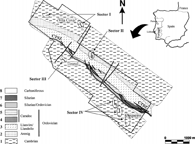
Figure3. Simplified geologicalmap of thestudied area (modified fromGon¸calves,1996), and itsgen-
erallocationin the inset map of the IberianPeninsula.Legend:1,Schistsandgreywackes;2, Quartzites;
3, Black shales; 4, Quartzites; 5, Shales and greywackes; 6, Undifferentiated Silurian and Ordovician
rocks; 7, Blackshales and cherts; 8:Carboniferous continental sediments (withcoal beds). Shear zones
as heavy solid lines; CTSZ: Carboniferous Trough Shear Zone. The elliptic areas correspond to the
main gold/antimony anomalies, where the inner black lines represent the main quartz vein directions
(overexaggerated). In sector III, the indicated structure is a minor shear zone parallel to the CTSZ.
Blank elliptic areas represent anomalous zoneswith probable concealed structures. The polygonalarea
on the map delimits the soil geochemistry coverage.
The studied area is located in NW Portugal, about 70 km South of Porto,
in Arouca. The mineralization occurs within quartz veins whose development is
closelyrelated to the evolution of a major NW-SE shear zone bounding continental
Carboniferoussediments tothe NE,and knownas the Carboniferous Trough Shear
Zone (CTSZ). This shear zone has several branches being sometimes cut by late
N-S and NE-SW dextral faults (Fig. 3). It presents a complex evolution being
active since the first deformation phases of the Variscan orogeny (late Devonian),
until the later stages under more brittle regimes (Permian). There are four main
anomalous sectors identified by soil geochemistry surveys.Of these, sector IV was
shown to be the most important one. Sector I shows some peculiar structural and
mineralogical aspects and will not be considered, but the remaining sectors show
development of the veins during the late deformation phases, where most energy

P1: Vendor/FNV P2: FLF
Mathematical Geology [mg] PL235-228125 September 29, 2000 11:14 Style file version June 30, 1999
52 Gon¸calves
is dissipated through deformation along major NW-SE dextral shear zones (like
the CTSZ). Consequently, secondary structures were developed and induced the
opening of en
´
echelon N-S to N20E quartz veins, especially in sectors II and IV.
The primary mineralization comprises quartz I + arsenopyrite I + other sulfides
(now mostly oxidized). In a later brittle stage, N-S dextral faults develop, and
consequently the quartz-vein walls act as discontinuities where deformation is
preferentially concentrated. Brecciation of quartz increased porosity and favoured
theinput of later hydrothermal fluids responsible for the second mineralizing event
with quartz II + arsenopyrite II ± electrum ± pyrite ± chalcopyrite. The richest
goldgradeisalwaysobtainedwithintheselaterminordomains,mainlyrepresented
in sector IV.
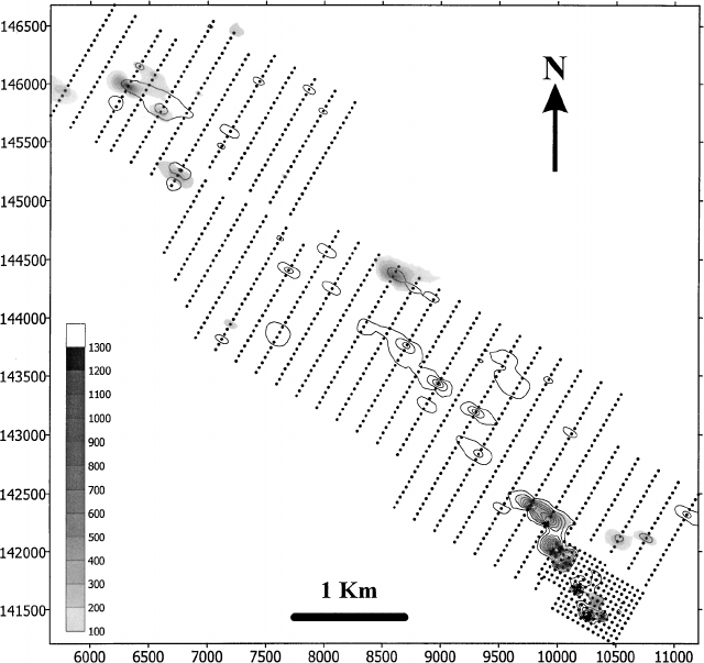
Figure 4 shows all 1187 sample locations, corresponding to two different
samplingsurveys: asmallareainthesoutheast(coveringpartofsectorIV)sampled
every 50 m, and the extension to a wider area with samples taken every50 m along
profiles 200 m apart. The total final area covered is 12 km
2
.
This area was overlain with a set of different grid sizes in order to perform a
multifractal study, using the method of moments. Grid sizes ranged from 200 m
(largest spacing between samples) to 800 m. Problems arose while using this
methodology, suchasedgeeffects,which brought some uncertaintytotheobtained
results, where errors accumulated very fast, especially for q > 0. There are other
promising methods to estimate the multifractal spectrum such as the method of
multipliers(Chhabra and Sreenivasan,1991) recently usedin geochemistry as well
(Cheng,1999).ThissortofproblemwasexaminedbyAgterbergand others(1996),
in which they used a modified version of Equation (5) to calculate the partition
function applied to a set of measured fracture lengths. These authors introduced
a weight fraction that is the ratio between the exposed cell area (or equivalently,
the cell area within the domain boundaries) and the total cell area. Accordingly,
Equation (5) becomes
χ
q
(ε) =
N
ε
X
i=1
w
i
µ
µ
i
w
i
q
, forq ∈< (30)
The weight in the ith cell is given by w
i
= s
i
/a
i
, where s
i
is the cell area within
the sample boundaries and a
i
is the total cell area. Equation (30) reduces to Equa-
tion (5) only when q = 1, assuming the measure in the area fraction of the cell is
representative of the entire cell. This assumption, however, is generally not true,
especially if there are very high or low values near the sampling boundaries. In
these situations, Equation (30) gives too much weight to these cells, and becomes a
considerable source of bias in the estimation of the multifractal spectrum. This can
be minimized either by a very large data set or setting a threshold of a minimum
P1: Vendor/FNV P2: FLF
Mathematical Geology [mg] PL235-228125 September 29, 2000 11:14 Style file version June 30, 1999
Characterization of Geochemical Distributions Using Multifractal Models 53
Figure 4. Plot showing geometry of the sampling grid and the spatial distribution of gold (greyscale
areas) and arsenic (contour lines). Greyscale for gold in ppb, and contour intervals for arsenic every
100 ppm (minimum contour 100 ppm). The coarse grid has profiles 200 m apart. Along the profiles
samplesweretakenevery 50 m. Thesmalldomaininthesoutheast corresponds to the earlier sampling
survey, with a finer grid. Geology has been omitted for clarity (Fig. 3) and the coordinates are in
meters.
cell area fraction considered for estimation, similar to what was done by Agterberg
and others (1996). Because very largedata sets are rare in the earth sciences, one is
left with the second possibility. Since several analyses were below detection limit,
e.g., gold and antimony (the most significant economic elements in the area) cor-
responding to circa 40% and 60% of the total analysis, respectively, only arsenic
values were used in this study. Out of the total number of samples, only 31 of
these were below detection limit (10 ppm), which corresponds to ≈2%, and these
points were not used for computation. Arsenic has a positive correlation with gold
as the hosted gold-quartz veins have significant amounts of arsenopyrite, and the

P1: Vendor/FNV P2: FLF
Mathematical Geology [mg] PL235-228125 September 29, 2000 11:14 Style file version June 30, 1999
54 Gon¸calves
Table 1. Estimated Values of the Mass Exponent τ(q) with Uncertainty Expressed as ±2σ (Estimated
Using Least Squares), for the Values of Arsenic in Soils; −3 ≤ q ≤ 3 with 0.5 Interval Increment
Area Fraction ξ
0 0.1 0.2 0.3 0.4
q τ (q) ±2στ(q)±2στ(q)±2στ(q)±2στ(q)±2σ
−3−9.222 0.027 −9.222 0.027 −9.223 0.027 −9.223 0.027 −9.226 0.026
−2.5 −8.002 0.019 −8.002 0.019 −8.002 0.019 −8.002 0.019 −8.008 0.019
−2 −6.783 0.013 −6.783 0.013 −6.783 0.013 −6.785 0.013 −6.793 0.013
−1.5 −5.569 0.008 −5.569 0.008 −5.570 0.008 −5.572 0.008 −5.585 0.009
−1 −4.364 0.005 −4.364 0.005 −4.365 0.005 −4.370 0.005 −4.389 0.006
−0.5 −3.171 0.002 −3.171 0.002 −3.174 0.002 −3.182 0.004 −3.211 0.005
0 −2.000 0.000 −2.000 0.000 −2.005 0.001 −2.019 0.004 −2.060 0.005
0.5 −0.861 0.002 −0.861 0.002 −0.870 0.003 −0.893 0.004 −0.950 0.006
1 0.226 0.006 0.226 0.006 0.212 0.006 0.175 0.006 0.099 0.010
1.5 1.236 0.013 1.236 0.013 1.210 0.011 1.157 0.010 1.059 0.016
2 2.145 0.027 2.145 0.027 2.099 0.019 2.026 0.018 1.906 0.025
2.5 2.954 0.051 2.954 0.051 2.877 0.029 2.782 0.029 2.640 0.039
3 3.689 0.087 3.689 0.087 3.568 0.043 3.449 0.043 3.288 0.056
different generations of this sulfide are consistent with the findings that two main
mineralizing events occur in the region (Gon¸calves, 1996). Scattered medium to
high values of arsenic (as well as gold) appears related to small veins and fractures
in the area as well, which may be verified by the spatial distribution of arsenic
(Fig. 4).
Equations(30),(6),(10),and(11)wereusedto computethe f (α) curvefor the
arsenic data. To deal with edge effects, severalthreshold valuesξ for the minimum
area fractions used to compute the partition function in Equation (30) were tested
to infer the quality of the obtained results. These threshold values were ξ = 0,
0.1, 0.2, 0.3, and 0.4, and grid cells with area fractions below ξ within the sample
area were discarded from computation. A summary of the results is presented
in Table 1 for arsenic, with the estimated values of ˆτ (q) for −3 < q < 3, and the
uncertaintyexpressedas±2σ .The chosen thresholdvaluetakes into consideration
that τ (0) =−2, since for q = 0, f (α) is at its maximum and is equal to D
0
, with
τ (1) = 0, as required for total mass conservation.
A brief inspection shows that ˆτ (0) deviates as ξ increases but ˆτ (1) approaches
the expected value. For area fractions below 0.3, the estimated values for ˆτ (1)
deviate significantly from what would be expected, thus violating the principle
of conservation of total mass. For other q values, the estimated ˆτ (q) deviates
differently depending on whether q is positive or negative. For q > 0, and for
differentareafractions,thecomputed ˆτ (q)deviatemorethantheuncertaintyrelated
P1: Vendor/FNV P2: FLF
Mathematical Geology [mg] PL235-228125 September 29, 2000 11:14 Style file version June 30, 1999
Characterization of Geochemical Distributions Using Multifractal Models 55
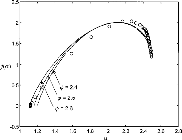
Figure 5. The f (α)—α curve for the arsenic soil data. A multifractal spectrum was obtained
using an area fraction ξ = 0.3 and computed for −15 ≤ q ≤ 10 (for all models) with a 0.5 step
increment. The spectrum of the model was computed with the enrichment factors φ indicated
and K
1
= 1.3.
to its own estimation. This means that the method is not robust and the accepted
values must be used with care. With that same range for q, and for area fractions
below 0.3 a deviation from linearity in Equation (6) is also observed. For q < 0,
the measure is considered robust since its difference is less than the uncertainty
of the estimations. Therefore, the threshold used was ξ = 0.3 as a compromising
solution.
The multifractal spectrum for arsenic was plotted together with some curves
of different model parameters (Fig. 5), and the general fit may be considered
reasonable. The constant K
1
= 1.3 is equal for all curves in Figure 5, and the
enrichment factors used are φ = 2.4, 2.5, and 2.6. The extreme points of the
left-sided part of the multifractal spectrum for the data are meaningless due to
error propagation. It is also worth noting that the different model curves for q >
0 follow the general trend for the data and are very close to the experimental
points. For each q, the arsenic data reaches 0 very rapidly due to the existence
of very high values in the distribution and lack of a representative number of
intermediate values. For q < 0, the data points and the model curves do deviate
P1: Vendor/FNV P2: FLF
Mathematical Geology [mg] PL235-228125 September 29, 2000 11:14 Style file version June 30, 1999
56 Gon¸calves
but agree closely in the f (α) range related to each considered q value. This is a
consequence of the large number of lowvalues of arsenic in the distribution,which
is consistent with the local background for this element of approximately 90 ppm
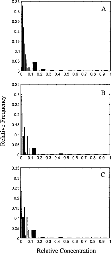
in the area (Gon¸calves, 1996). Comparative histograms for the real data and model
were constructed and shown in Figure 6. All concentrations were normalized to
their maximum concentration so that the distributions could be compared. Model
concentrations were generated with φ = 2.5, K
1
= 1.3, and n = 5 (fifth-order
cells). Distributions differ mostly in the lower values (less than 0.1), where the
generated data showsspikesin some classes of concentrations. In the exampledata
set, a decrease in frequency is observed for each class of concentrations up to 0.1.
A major differenceappears in the first class of concentrations, which in the arsenic
data corresponds to the values close to the detection limit. Such a truncation is not
a model property, where a continuum of concentrations may be ideally achieved
as long as n →∞. However, setting a relative detection limit identical to the
real data set did not improve the model significantly (Fig. 6C). Values of relative
concentration greater than 0.1 are replicated fairly well, which justifies the closer
agreement between both model and experimental multifractal spectrums (Fig. 5).
Noticeable differences are observed in the frequencies of concentrations in the
intervals (0.2,0.3], and (0.4,0.5].
Another way to test model fitness to data would be the use of the q/D
q
plot (Fig. 2) but this proved to be less sensitive than the multifractal spectrum
in highlighting the differences (here referring to q < 0). Another problem arises
because of Equation (7), and that is the uncertainty in the estimates of τ (q) for
q > 0, especially close to 1 that make the D
q
estimation to diverge for q → 1, in
particular
ˆ
D
q
→−∞as q → 1−, and
ˆ
D
q
→+∞as q → 1+.
The proposed model may closely characterize at least some geochemical
distributions,providedthat the whole population is sufficientlyrepresented in both
extremesof the range of values. Therefore, in this case, the enrichment factor gives
themagnitudeoftheefficiencyoftheconcentrationprocessinrelationtotheglobal
average of arsenic present in the soils, which may attain a maximum concentration
of 1280 ppm. On the other hand, the K
1
constant may model the distribution of the
lower arsenic concentrations in the several small scattered veins that appear in the
sampled area, generally in the range of 200–500 ppm in the rocks. Examples of
these small structures are the lower value anomalies close to the sheared Caradoc
quartzites between sectors II and IV, and just to the north of sector IV as well
(Figs. 3 and 4). These last areas have correspondingly smaller concentrations in
the soils, down to 90 ppm, which represents the local background.
The existence of irregularly spaced data often implies the need for interpola-
tion of values onto a regular grid, which can be done via, e.g., kriging. Ordinary
lognormal kriging was used to estimate arsenic values,here followingthe method-
ology of Journel and Huijbregts (1978), interpolating a point every 100 m and
producing a more regular grid in order to test the differences in the multifractal
P1: Vendor/FNV P2: FLF
Mathematical Geology [mg] PL235-228125 September 29, 2000 11:14 Style file version June 30, 1999
Figure 6. Histograms showing the relative frequencies of
arsenic concentrations in the example data set, A, and of
the generated concentrations using the proposed model with
n = 5, φ = 2.5, and K
1
= 1.3, B and C. Concentrations were
normalized, in each case, to their respective maximum value.
In C, alowercut-offvalueequal to therelative detection limit
of the example data set was assumed. The interval width of
each class is 0.01 between 0 and 0.1, and is 0.1 between 0.1
and 1.
57

P1: Vendor/FNV P2: FLF
Mathematical Geology [mg] PL235-228125 September 29, 2000 11:14 Style file version June 30, 1999
58 Gon¸calves
Table 2. Estimated Values of the Mass Exponent τ (q) with Uncertainty Expressed as ±2σ
(Estimated Using Least Squares), for the Values of Arsenic Estimated with Lognormal Kriging over a
Regular Grid of 100 × 100 m; −3 ≤ q ≤ 3 with 0.5 Interval Increment
Area Fraction ξ
0 0.1 0.2 0.3 0.4
q τ (q) ±2στ(q)±2στ(q)±2στ(q)±2στ(q)±2σ
−3−8.529 0.019 −8.529 0.019 −8.529 0.019 −8.529 0.019 −8.531 0.018
−2.5 −7.414 0.014 −7.414 0.014 −7.414 0.014 −7.414 0.014 −7.416 0.014
−2 −6.309 0.010 −6.309 0.010 −6.310 0.010 −6.311 0.010 −6.313 0.010
−1.5 −5.216 0.007 −5.216 0.007 −5.217 0.007 −5.218 0.007 −5.222 0.007
−1 −4.134 0.004 −4.134 0.004 −4.135 0.004 −4.139 0.004 −4.144 0.004
−0.5 −3.062 0.002 −3.063 0.002 −3.067 0.002 −3.074 0.002 −3.081 0.002
0 −2.000 0.000 −2.001 0.000 −2.011 0.001 −2.025 0.002 −2.036 0.002
0.5 −0.938 0.002 −0.941 0.001 −0.967 0.003 −0.995 0.004 −1.010 0.003
1 0.144 0.006 0.134 0.004 0.070 0.007 0.015 0.007 −0.008 0.005
1.5 1.284 0.016 1.253 0.012 1.105 0.016 1.003 0.011 0.967 0.009
2 2.533 0.037 2.449 0.026 2.146 0.033 1.965 0.016 1.912 0.014
2.5 3.913 0.071 3.730 0.047 3.192 0.056 2.901 0.023 2.819 0.021
3 5.390 0.114 5.067 0.070 4.237 0.085 3.805 0.030 3.683 0.028
spectrumoftheestimateddata.Thenumberofpointsalongtheprofileswasreduced
to half, and was reduced in both directions in the southeast part of the sampled
area. Since the original grid is not exactly regular, the estimated points rarely
coincide with the original data points, but are normally close to some known
point. To compute the partition function, the area fraction used was againξ = 0.3,
essentially for the same reasons as discussed earlier. Table 2 shows that ˆτ (1) is
closer to the predicted value for the considered ξ ; however, for higher q values
the estimation of the mass exponent has exactly the same problem as the previous
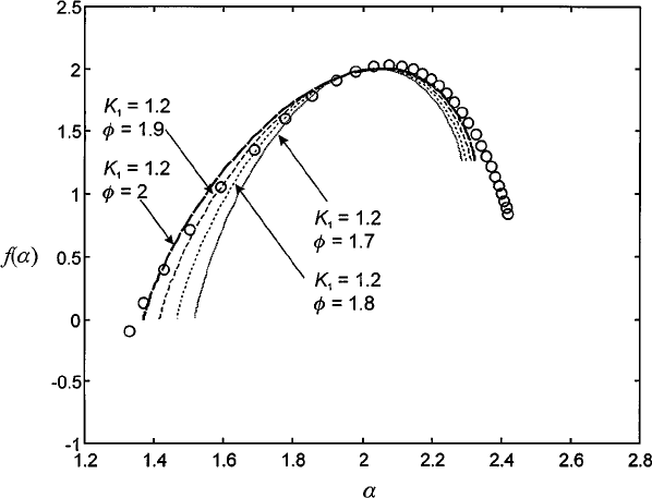
exampleinthispaper.Whenestimatedvalues wereusedtocalculate itsmultifractal
spectrum,it wasfound to be in good agreement with someof the model parameters
(Fig. 7), especially for φ = 2 and K
1
= 1.2. The multifractal spectrum is different
fromtheoriginaldataset, mainlybecauseinterpolatingafullrowofpointsbetween
each profile smoothes the data. The extreme values for higher q values are reduced
through the same smoothing effect, and agreement on this side of the curve is
very good. The curves for φ between 1.7 and 1.9 are also close to the data set and
are plotted for comparison. The fit is worse for the negative q side of the curve,
and fails to reproduce the whole spectrum of values. Fitting a model with a lower
enrichment factor and a lower value for the K
1
parameter shows that the estimated
points are a smoothed version of the original data points. Therefore, use of the
multifractal spectrum together with a good model for the data set may become a
useful tool for the stochastic modeling of geochemical distributions.
P1: Vendor/FNV P2: FLF
Mathematical Geology [mg] PL235-228125 September 29, 2000 11:14 Style file version June 30, 1999
Characterization of Geochemical Distributions Using Multifractal Models 59
Figure 7. Multifractal spectrum for the interpolated arsenic values on a 100 × 100 m grid
(−10 ≤ q ≤ 5). Kriging smoothed the interpolated values to a distribution very close to one
characterized by an enrichment factor φ = 2 and K
1
= 1.2(−10 ≤ q ≤ 10). Curves for φ =
1.9, 1.8, and 1.7 are shown for comparison.
CONCLUSIONS
In the present paper, a two-dimensional multifractal model based on a trino-
mial multiplicativecascade was proposed as a proxy to some kinds of geochemical
distributions. It was noted that this is just one of many possible models that may
be constructed, some of which may also be much closer to real distributions. In
any case, this opens a possible line of research for the use of such approaches in
geochemical modeling.
Itwasshownthatinrelationtotheexampledataset,theproposedmodelcould
characterize the distribution fairly well. The number of model parameters may be
increased to improve the fit to a larger range of distribution types but this also
increasesthe mathematical complexity, andthe derivationof the equations become
much more difficult and harder to handle. These equations have been derived for
the proposed model inorder to compute the multifractal spectrum with the desired
accuracy. The objective was to compare the f (α) curve of the model with real
data, giving an approximate generating mechanism for the studied data, and try to
P1: Vendor/FNV P2: FLF
Mathematical Geology [mg] PL235-228125 September 29, 2000 11:14 Style file version June 30, 1999
60 Gon¸calves
relate the model parameters with the mechanisms responsible for the dispersion
and concentration of chemical elements. Such comparison must consider not only
the curve itself but also the range of q values used for the computation.
The distribution of arsenic in soils in an area with gold mineralizations was
used as an example. In performing a multifractal analysis on this data, problems
with the computation of the partition function and the estimation of the mass
exponent arose as a consequence of the difficulty of subdividing an area with
several boxes of regular side length. The edge effects were always an important
source of bias in the estimations and must be evaluated carefully. It has been
shown that the model produces a reasonable fit for the distribution studied using
enrichmentfactorsintherangeof2.4–2.6and K
1
= 1.3.Therefore,theenrichment
factor can give an estimate of the concentration efficiency in the main mineralized
structures in relation to its global average concentration in the whole area. It is
not possible to draw a relation between the number of mineralizing events and the
generation order n of the model used to generate the histograms with theclosest fit
to the arsenic concentrations, in spite of the various metasomatic events identified
in these deposits. Such a relation would certainly give the enrichment factor a
more quantitative and predictable basis, provided the host rocks act as possible
sources of the chemical elements, and these are preferentially concentrated in one
area. The K
1
constant provides a picture of the heterogeneity of the distribution,
mainly represented by the small-scattered quartz veins in the studied area. The
same procedure was done for the values estimated from the example data set. In
this case, fitting a lower enrichment factor essentially showed that these values
were a smoothed version of the original data.
Similar studies may be very important to improve future models that may
include a much wider set of distributions, and provide the philosophy underneath
its construction. On the other hand, these approaches may act as an alternative
tool for the stochastic simulation of geochemical distributions. However, more
extensive testing on other data sets will be required to evaluate to what extent
these models may be truly useful for the study, and even the understanding, of
geochemical distributions.
ACKNOWLEDGMENTS
The author wishes to acknowledge Empresa de Desenvolvimento Mineiro,
SA (EDM) for providing thesoil geochemistry data set of Cons´orcio Baixo Douro
(EDM/BRGM/ECD).ThecolleagueAnt´onio Mateus is also acknowledgedforthe
careful review of an earlier version of this paper and the stimulating discussions on
the esoteric (to the earth scientists) stuff of fractals. Susana Nascimento gave in-
valuablesuggestions on the mathematical presentation. Andreas Prokoph, Bradley
Sim, and an anonymous reviewer are greatly acknowledged for their comments
that help to improve and clarify the present paper.