Graebel W.P. Advanced Fluid Mechanics
Подождите немного. Документ загружается.

174 The Boundary Layer Approximation
being locally normal to the boundary, the equations still hold, since curvature effects
are of higher order unless the curvature is extreme.
In approximating the Navier-Stokes equations by the boundary layer equations,
the mathematical character of the equations have changed. The original Navier-Stokes
equations are of elliptic nature, while the boundary layer equations are parabolic. (The
boundary layer equations are sometimes referred to as the parabolized Navier-Stokes
equations.) Equations of parabolic type have solutions that can be “marched” in the
x direction, and the numerical methods appropriate for parabolic equations are quite
different from those used for elliptic equations. The implication now is that upstream
conditions completely determine downstream behavior. When this is not true, for exam-
ple, where a flow starts to separate, the boundary layer assumption breaks down.
6.3 Boundary Layer Thickness
In Chapter 5 where exact solutions were being considered, boundary layer thickness
was established by first finding the solution and then considering for what value of
the horizontal velocity component approached some percentage of the outer velocity.
For both theoretical and experimental purposes, it is preferable to have a less subjective
definition of “thickness.” Two such definitions have been found to be useful.
The displacement thickness of the boundary layer is defined by
D
=
1
U
0
U −udy = displacement thickness (6.3.1)
where is a value “large enough” so that choosing a slightly larger value would not
significantly affect the value of
D
. Looking at Figure 6.4.1 (on page 177), we can
see that the integral represents the area U minus the actual discharge in the layer of
thickness . As the value of is increased, there comes a point where no significant area
is added to the integral, so whether 90%, 99%, or evaluation by eye of experimental
data is used, the value of the displacement thickness remains virtually unchanged.
Another interpretation of the displacement thickness is that because the volumetric
flow in the boundary layer is actually
0
udy, the same flow would be achieved if the
wall was displaced upward into the flow in an amount
D
, since the definition can be
written in the form
−
D
U =
0
udy
Similarly, a momentum thickness definition has been found to be useful. It is
given by
M
=
1
U
2
0
uU −udy = momentum thickness (6.3.2)
Again, its value is relatively insensitive to increases in as long as a large enough
is chosen. Its physical interpretation is a bit more difficult to explain than the previous
definition, as it involves the momentum difference between the actual flow and an
inviscid one with the same discharge, as follows from
U
0
udy −U
2
M
=
0
u
2
dy
As we will see in Section 6.5, both these quantities arise naturally when the boundary
layers are integrated over the boundary layer thickness.
6.4 Falkner-Skan Solutions for Flow Past a Wedge 175
6.4 Falkner-Skan Solutions for Flow Past a Wedge
To illustrate the behavior of the boundary layer equations, next consider a solution of
similarity type first credited to Falkner and Skan (1930). This is a solution where U
is proportional to x
m
. The irrotational flow that corresponds to this is the flow past a
wedge of angle radians with a complex potential and velocity given by
w = +i =
Az
m +1
m +1
=
Ar
m +1
cos
m +1
+i sin
m +1
m +1
(6.4.1)
dw
dz
=u −iv = Ar
m
cosm +i sin m
(6.4.2)
Evaluating equation (6.4.1) on the surface of the wedge = 0 gives U = Ax
m
. From
the Euler equations,
−
p
x
=U
dU
dx
=mA
2
x
2m −1
For the similarity form of the solution use
=
Ux/f with =y
U/x
as in the full Navier-Stokes equations. Then with
x
=
m −1
2
x
d
d
y
=
U
x
d
d
from differentiation of find that
u =Uf
v=−
1
2
U
x
m +1f +m −1f
u
x
=
U
x
mf
+05m −1f
u
y
=U
U/xf
2
u
y
2
=
U
2
x
f
Substituting all of these into the boundary layer equations, the result is
m
f
2
−05m +1ff
=m +f
The terms on the left-hand side result from the convected acceleration, the constant on
the right side results from the pressure gradient, and the third derivative is the viscous
stress gradient. Rearranging to put all terms on the left-hand side, the result is
f
+05m +1ff
+m1 −f
2
=0 (6.4.3)
Equation (6.4.3) is to be solved together with the no-slip boundary conditions
f0 = f
0 = 0 (6.4.4)
and the outer condition
f
approaches 1 as becomes large (6.4.5)
The shear stress at the wall is
wall
=
u
y
y =0
=U
U/xf
0 (6.4.6)
Consider next several special cases of equation (6.4.6).
176 The Boundary Layer Approximation
6.4.1 Boundary Layer on a Flat Plate
The first solution of equation (6.4.3) was carried out by Blasius (1908) for a semi-infinite
flat plate, where m =0. Then equation (6.4.3) reduces to
f
+05ff
=0 (6.4.7)
Equation (6.4.7) has the minimum number of terms that equation (6.4.3) can have for a
boundary layer flow, but still no exact solution is possible. A numerical solution must
be resorted to, and since boundary conditions must be applied at both the wall and the
outer edge of the boundary layer, generally our choice is either to use a shooting method
(first guess f
0, then integrate out from the wall to see if f
approaches unity, then
iterate on this procedure) or use a two-point method that has the boundary conditions
at both ends included. Blasius found that f
0 = 0332.
For this special problem only, numerical integration using a shooting method can
be simplified. First, make the change of variables =c and f =cF so that equation
(6.4.7) is replaced by
F
+05FF
=0 (6.4.8)
where this time a prime is a derivative with respect to .
Set F
0 arbitrarily to unity, and integrate to find that F
approaches some value
b at large . Then, letting c = 1/
√
b will make f
approach unity as becomes large,
completing the desired solution. The results of such a numerical integration are shown
in Table 6.4.1 and Figure 6.4.1.
Several interesting features of boundary layer flows can be seen from the results of
this problem.
1. Since the outer edge of the boundary layer is at some constant value of , the
exact value depending on how the boundary layer thickness has been defined,
then ∼x/
√
Ux/.
2. As becomes large, f approaches the asymptotic value −17208. Thus, the
displacement thickness is
D
=
1
U
0
U −udy =17208x
/Ux
3. The shear stress is proportional to x
−1/2
, so the shear stress decreases going
downstream from the plate leading edge. This decrease is due to the thickening
of the boundary layer, with a resulting decrease in velocity gradient.
4. The drag force per unit width over a length L of the plate is
F =
L
0
wall
dx = 2Uf
0
UL/
5. From the asymptotic value of f , the stream function is seen to approach
= Uy −17208
Ux/ +···
Thus, the displacement thickness effect does not result in an irrotational flow
away from the wall.
6.4 Falkner-Skan Solutions for Flow Past a Wedge 177
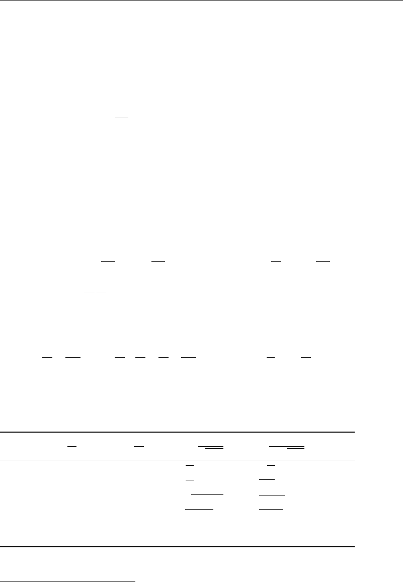
TABLE 6.4.1 Flat plate boundary layer (Blasius)
f f
f
f f
f
0000000 00000 03320 2006500 06298 02668
0100017 00332 03320 2207812 06813 02484
0200066 00664 03320 2409223 07290 02281
0300149 00996 03318 2610725 07725 02065
0400266 01328 03315 2812310 08115 01840
0500415 01659 03309 3013968 08460 01614
0600597 01989 03301 3215691 08761 01391
0700813 02319 03289 3417469 09018 01179
0801061 02647 03274 3619295 09233 00981
0901342 02974 03254 3821160 09411 00801
1001656 03298 03230 4023057 09555 00642
1102002 03619 03201 4209670 24980 00505
1202379 03938 03166 4426924 09759 00390
1302789 04252 03125 4628882 09827 00295
1403230 04563 03079 4830853 09878 00219
1503701 04868 03026 5032833 09915 00159
1604203 05168 02967 5537806 09969 00066
1704735 05461 02901 6042796 09990 00024
1805295 05748 02829 6547793 09997 00008
1905884 06027 02751 7052792 09999 00002
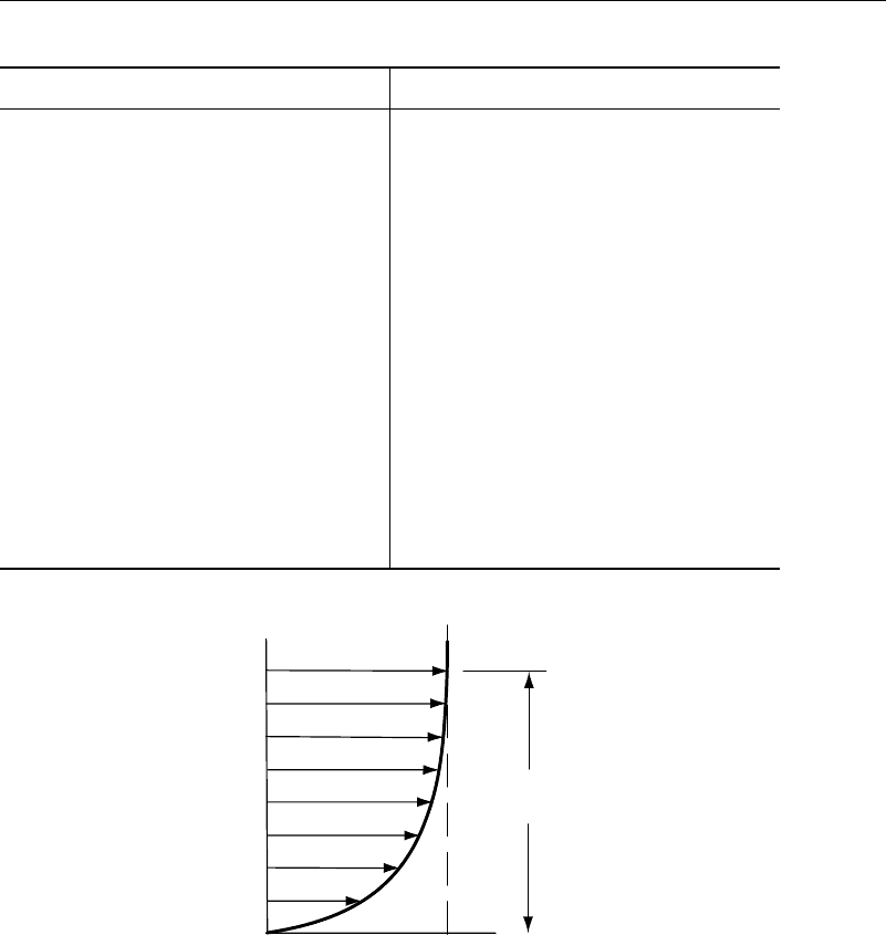
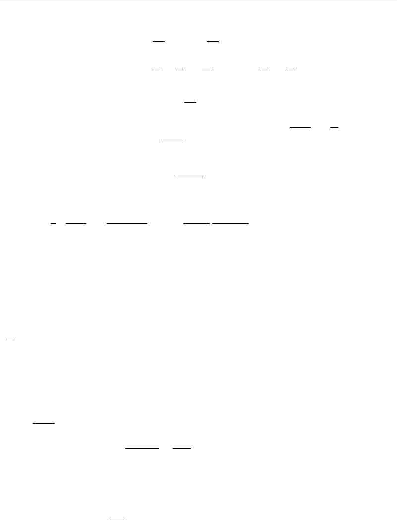
u
U
δ
y
Figure 6.4.1 Blasius’s solution for boundary layer flow on a semi-infinite plate
6. The shear stress is infinite for all values of y at x =0. We could be content with
this if it were infinite only at the leading edge, but it is perhaps surprising that it
should be singular along a line perpendicular to the plate. Also, a solution does
not exist for negative x, for in that case becomes imaginary.
The criticisms raised in the last two points may seen to be minor ones, but they are
needless errors that have in fact been introduced by our choice of a coordinate system.
In performing any mathematical solution, it is always best to use a natural coordinate
system (Kaplun, 1954)—that is, one where setting one of the coordinates to a constant
value yields the desired boundary. For our choice of a coordinate system, the boundary
is at y =0 for x>0.
178 The Boundary Layer Approximation
Having to qualify the value of x by saying that it must be positive means that this
is not a natural coordinate system for this problem. A coordinate system that is a natural
coordinate system for the semi-infinite flat plate is a parabolic system, given by
2
=x +
x
2
+y
2
2
=−x +
x
2
+y
2
(6.4.9)
with the inverse relations
x =
2
−
2
2
y= (6.4.10)
Use of these coordinates eliminates both problems raised in points e and f , leaves
equation (6.4.7) unchanged so the problem does not have to be re-solved, and the
parabolic behaves as the originally introduced, since far away from the leading
edge along the plate it is seen that
√
2x y/
√
2x.
You may have noticed another point that involves general principles in what has
been done. In deriving the boundary layer approximation in the first place, it was stated
that there was a definite boundary length scale L upon which our Reynolds number was
based. In the Falkner-Skan problems, however, there is no such L, and our results come
out with a Reynolds number based on the local distance x. The distinction is perhaps
subtle, but it is important as far as an understanding of the implications is concerned.
The question was not answered until the 1960s, and the lack of attention to the problem
resulted in some confusing and erroneous publications prior to that time.
When there is a fixed-length scale L in a problem, what is being done in the
boundary layer approximation is expanding the solution to the Navier-Stokes equations
in terms of negative powers (and perhaps logarithms) of the Reynolds number. This is
then an expansion in the constant parameter Re. Near a boundary, the first term in the
expansion is the boundary layer equation.
Away from boundaries, the first term in the expansion is the Euler equation.
Presumably, it is possible to go to higher-order terms in the expansion (albeit with
increasing difficulty and work) and still have the solutions match at the overlap of the
Euler and boundary layer regions.
When there is no geometric length scale L, the expansion is in terms of a coordi-
nate such as x, but it may not be able to find solutions in the various regions that
mathematically match together properly, although they might numerically join together
satisfactorily. The question of how to obtain higher-order approximations is thus left
unanswered, and we may have to be satisfied with just the lowest-order approximation.
(We usually settle for this in any case, but it would be nice to at least know that
higher-order approximations could be carried out if we wanted them.) A more thorough
discussion of this matter can be found in Van Dyke (1964).
6.4.2 Stagnation Point Boundary Layer Flow
When = , the inviscid flow becomes flow perpendicular to a flat plate, and our
equation reduces to that found in the full solution of the Navier-Stokes equations. In
this case, then, the boundary layer solution is an exact solution of the Navier-Stokes
equations for the velocity (but not the pressure).
6.4.3 General Case
Values for f
0 are given in Table 6.4.2 for a number of wedge angles. The last
18 sets of values in were computed by Hartree in 1937. He found that if >0, the

6.5 The Integral Form of the Boundary Layer Equations 179
TABLE 6.4.2 f
0 as a function of and m
mf
0
radians degrees
−056549 −324 −008257 −00657
−047124 −27 −006977 −009002
−031416 −18 −004762 −00973
−015708 −9 −002439 −007543
−007854 −45 −001235 −0052
−062202 −3564 −009008 0
−059692 −342 −008676 005811
−05655 −324 −008257 00871
−050262 −288 −007407 012928
−043982 −252 −006542 016338
−031417 −18 −004762 022013
000 033206
031415 18 005263 042585
062831 36 011111 051131
094248 54 017647 059363
125664 72 025 067586
157078 90 033333 075689
188495 108 042857 084177
251312 144 066667 10224
314159 180 1 12326
376991 216 15149669
502655 288 4 240491
628318 360
solution of equation (6.4.7) was unique and that for >20, the velocity components
are imaginary. He carried the solution out for = 24 to facilitate interpolation and for
values of <0 for which f
approached one exponentially from below.
Stewartson (1954) computed the first five values in the table. These flows show
reversed flow regions near the wall and also demonstrate that for a given value of m,
the solution of equation (6.4.3) is not necessarily unique.
The fact that solutions of the Falkner-Skan equation may not be unique is interesting
in itself. It also is a caution that simply formulating a similarity solution in terms of a
nonlinear ordinary differential equation along with appropriate boundary conditions is
not the end of the story. At least one solution must be found and then investigated over
at least some useful parameter range so that there is reasonable cause to believe that
there are no other solutions for those parameters.
6.5 The Integral Form of the Boundary Layer Equations
Next, an integral form for the boundary layer approximation will be derived by inte-
grating the boundary layer equation. First, rearrange equation (6.2.14) in the form
U −u
t
+U
U
x
−u
u
x
−v
u
y
=−
2
u
y
2
(6.5.1)
180 The Boundary Layer Approximation
From integration of the continuity relation equation (6.2.16), find that
v
=−
0
u
x
dy (6.5.2)
Integrating equation (6.5.1) with respect to y and using the continuity equation and the
product rule of calculus, the result is
wall
=
0
U −u
t
+U
U
x
−u
u
x
−v
u
y
dy
=
U
D
t
+
0
U
U
x
−u
u
x
−
uv
y
+u
v
y
dy
=
U
D
t
+
0
U
U
x
−2u
u
x
+u
u
x
+
v
y
dy −Uv
Using equation (6.5.2) to bring the last term back under the integral sign gives
wall
=
U
D
t
+
0
U
U
x
−
u
2
x
+U
u
x
dy
=
U
D
t
+
0
U
U
x
−
u
2
x
+
Uu
x
−u
U
x
dy
=
U
D
t
+
0
U
x
U −u
+
x
u
U −u
dy
=
U
D
t
+U
U
x
D
+
U
2
M
x
(6.5.3)
To use equation (6.5.3) to estimate the nature of the boundary layer a form for uy
must be chosen. For illustration of the method, choose first a linear approximation,
uy =
⎧
⎨
⎩
U
y
0 ≤ y ≤
U y ≥
Then,
D
= 05,
D
= 0167, and
wall
= U/. Inserting these into equation
(6.5.3) gives
U
=
t
05U
+05U
U
x
+
x
0167U
2
Multiplying this by gives
U
=
t
025U
2
+05U
2
U
x
+
x
00835U
2
2
Provided U is known, this is a linear equation in
2
. For the case of the steady flow past
a flat plate it reduces to U / = d/dx
00835U
2
2
, giving =
x/00835U =
346x
√
/xU.
We can see that this has the correct Reynolds number dependency. Using this to
determine the shear stress gives
wall
=
U
346
√
x/U
=0289U
2
Ux
6.5 The Integral Form of the Boundary Layer Equations 181
Again, the Reynolds number behavior is correct, and the 0.289 is only 13% apart from
the Blasius value of 0.332.
The linear approximation used here is, of course, unnecessarily crude. Other profiles
that could have been used follow, where =y/:
Parabolicu=
U
2 −
2
0 ≤ ≤ 1
U ≥1
Sinusoidalu=
U sin
2
0 ≤ ≤ 1
U ≥ 1
(6.5.4)
Pohlhausenu=
U
2 −2
3
+
4
+2
−3
2
+3
3
−
4
0 ≤ ≤ 1
U ≥1
The results for the flat plate are given in Table 6.5.1.
The Pohlhausen profile
1
(1921) was selected to agree with all solutions that were
known by 1921. Pohlhausen used the following boundary conditions in the selection
process:
At =0u= 0
2
u
y
2
=−U
dU
dx
At =1u= U
u
y
=0
2
u
y
2
=0
The parameter =
2
dU
dx
must lie in the range −12 ≤ ≤ 12, since at =−12 the
shear stress becomes zero at the wall, implying flow separation, and at =12 becomes
greater than U within the boundary layer.
If the Kármán-Pohlhausen approximation is inserted into our equations, the result is
D
=
3
10
−
120
M
=
63
37
5
−
15
−
2
144
and
wall
=2
U
1+
12
(6.5.5)
TABLE 6.5.1 Comparison of various boundary layer profiles with the Blasius results
Velocity
Profile
D
M
√
x/U
wall
U
√
U/x
Error in
wall
Linear 1/2 = 051/3 = 0167
√
12 = 346 1/
√
12 = 0288 13%
Parabolic 1/3 = 0333 2/15 = 0133
√
30 = 548
2/15 = 0365 9.9%
Sinusoidal 1 −2/ =0363 2/ −1/2 =0137
2/4 − = 48
√
2 −/2/2 =0 328 1.5%
Kármán-
Pohlhausen
0.3 37/315 =0117
1260/37 = 5836
37/315 = 0343 3.3%
Blasius 0.344 0.1328 5.0 0.332 0%
1
Pohlhausen was acting on a suggestion by von Kármán (1921), so the method is usually referred to as
the Kármán-Pohlhausen method.
182 The Boundary Layer Approximation
Putting these into the integrated Navier-Stokes equations results (after a reasonable
amount of algebraic manipulation) in
U
d
2
M
dx
=HK where
FK =
D
M
=
63
3−/12
10
37/5−/15−
2
/144
GK =
M
U
u
y
wall
=
2
63
1+
12
37
5
−
15
−
2
144
HK =2GK −2K
2 +FK
K =
2
M
dU
dx
=
1
3969
37
5
−
15
−
2
144
2
(6.5.6)
While this looks formidable, plotting H versus K shows that over a good range the
relationship is practically linear and given by HK =047 −6K. Thus,
U
d
2
M
dx
≈047 −6K or
U
5
d
U
6
2
M
dx
≈047
After integration of this it becomes
2
M
=
2
M
0
+
047
U
6
x
0
U
5
dx (6.5.7)
As we will see in the next section, this result is useful in predicting separation.
Because of the present day availability of ready access to powerful personal com-
puters, the integral formulation of the boundary layer equations is no longer as important
as it once was. However, the integrated form of the boundary layer is still convenient
for providing an approximate solution of the boundary layer equations with a minimum
amount of labor with reasonable accuracy. It is also useful for providing starting values
for the wall shear when more accurate numerical methods are used.
6.6 Axisymmetric Laminar Jet
Using the boundary layer equations, it is also possible to solve for a laminar jet, similar
to Squire’s solution in Section 5.4.5. Working in cylindrical polar coordinates, let
=
4z
f with =
1
8
r
z
3M
2
1/2
Here, M is the momentum of the jet given by
M =
0
w
2
2rdr (6.6.1)
The boundary layer momentum equation in the z direction then becomes, after a bit of
rearranging,
d
d
4f
df
d
=
d
d
1
df
d
−
d
2
f
d
2
(6.6.2)
6.7 Flow Separation 183
with the boundary conditions
f0 = 0
df
d
0
=0
df
d
=0 (6.6.3)
Integrating equation (6.6.2) gives 4f
df
d
=
df
d
−
d
2
f
d
2
. Since 4f
df
d
= 2
df
2
d
, this can be
integrated to give
2f
2
=2f −
df
d
+C
1
From the boundary conditions the constant of integration C
1
=0. Then
df
−f
2
+f
=2
d
.
This can be integrated to give f =
C
2
2
1+C
2
2
. Using equation (6.6.1) find C
2
= 1, so
finally
f =
2
1+
2
(6.6.4)
and
u =
1
2
3M
z
2
1/2
1−
2
1+
2
2
w=
3M
8z
1
1+
2
2
(6.6.5), (6.6.6)
6.7 Flow Separation
When the pressure gradient along a body surface is negative (favorable pressure gra-
dient), the pressure acts to locally accelerate the flow along the body and to overcome
the viscous forces that act to decelerate. However, when the pressure gradient becomes
positive (adverse pressure gradient), both pressure and viscous stresses act to decelerate
the flow, and the boundary layer thickness rapidly increases. The flow soon reverses
u
y
wall
< 0
, and flow separation is said to occur.
The point at which the flow reversal starts is called the separation point and is
usually a short distance downstream from the point where the pressure gradient changes
sign. Boundary layer theory is capable of predicting where the separation point is located
but is not able to predict the flow past this point.
Thwaites (1949) correlated a number of solutions of the integrated boundary
layer equations and found that separation could be closely predicted by the result
2
M
=−
009
dU/dx
. Inserting this into equation (6.5.7) gives
−
009
dU/dx
=
047
U
6
x
0
U
5
dx (6.7.1)
where the integration has been started from a stagnation point.
A second criteria suggested by Stratford (1954) suggests that separation will occur
at the point where
x −x
0
2
c
p
dc
p
dx
2
=00104 where c
p
=1 −U
2
/U
2
max
(6.7.2)
Both criteria require knowledge of U at the boundary. The Stratford criterion is some-
what easier to use in that it doesn’t involve an integration.
Even though the Thwaites and Stratford criteria are for two-dimensional flows, they
are frequently used in three-dimensions in situations where the flow is predominately
two-dimensional in behavior.