Graziani F. (editor) Computational Methods in Transport

Подождите немного. Документ загружается.

100 A.B. Davis

for the 1-point variability of the extinction coeﬃcient. Technically, the brack-

eted entity is a sub-set of M. In the random ﬁeld theory used here, we will

not need to distinguish “probability” per se from the normalized measure of

the set (in the sense of Lebesgue) where the values of interest occur.

In a uniform medium of extinction σ

Pr(dσ)=δ(σ − σ

)dσ. (59)

As a simple example of a variable medium, take a Bernoulli (binary-value)

random extinction

Pr(dσ)=[f

δ(σ − σ

)+f

δ(σ − σ

)]dσ, f

+ f

=1. (60)

We will however usually be dealing with continuous distributions of σ,hence

the diﬀerential notation.

“Ensemble” averages over this “disorder” in the optical medium will be

denoted by angular brackets, ·; so, for instance, we have

σ

 =

∞



Pr(dσ) . (61)

Statistical quantities of interest in photon transport are the ensemble-averaged

moments of the (random) FPD, equivalently, the moments of the ensemble-

average FPD

p(s) = dP (s)/ds. (62)

Speciﬁcally, we may want

E(s

) =

∞



dP (s) (63)

where

dP (s)/ds =

∞



p(s|σ)Pr(dσ)=

∞



σ exp[−σs]Pr(dσ) . (64)

So (63) is actually a double integral on probability measures: ﬁrst on the

spatial disorder, then on the propagation (as written above), or vice-versa.

Thinking of

τ(s)=σs (65)

when extinction σ is random and distance s ﬁxed, we are interested in the

statistical properties of the mean direct transmission law

e

−τ(s)

 =

∞



dir

(s|σ)Pr(dσ)=

∞



exp[−σs]Pr(dσ) . (66)

Eﬀective Propagation Kernels in Structured Media 101

In short, how does it diﬀer from e

−τ(s)

−σs

? From (66), we recover the

mean FPD in (64):

dP (s) =



e

−τ(s)





ds. (67)

Three general results can be derived about the mean or “eﬀective” FPD in

(64) or (66)–(67).

1. It is exponential only if the medium is homogeneous, a consequence of

Jensen’s inequality for f(X)=e

−X

. This is the converse of the result

derived in (43), thus making exactly exponential transmission and homo-

geneity equivalent statements about an optical medium:

σ(x) ≡ constant ⇐⇒



dir



∝ T

dir

. (68)

An important corollary here is that eﬀective medium (or homogenization)

theory is of limited value as an approach for 3D RT in the presence of

unresolved spatial variability. It is probably wise to customize the eﬀective

parameters of the uniform medium to deliver on some important aspect

of the problem at hand, rather than to think of it as a truly “equivalent”

medium.

2. The mean MFP is always larger than in the hypothetical homogeneous

medium with an extinction equal to the mean extinction; considering

(10), we are thus putting a number/mass-conservation constraint on the

variability. This translates to

 = E(s) = 1/σ≥1/σ . (69)

The inequality follows from Jensen’s in (57) for the convex function

f(X)=1/X. The local quantity 1/σ(x) is probably not equal to the

MFP deﬁned in (50) for any direction Ω. However, it is clearly a better

guess than the mean extinction σ. I will call the local quantity 1/σ(x)

the pseudo-MFP.

3. The mean FPD is always wider-than-exponential in the sense that its

higher-order moments are always under-estimated by assuming an expo-

nential distribution, even if we make a judicious adjustment for item 2

by using the actual MFP:

E(s

) = Γ (q +1)σ

−q

≥Γ (q +1)σ

−1



= Γ (q +1)

,q>1 . (70)

This follows from Jensen’s inequality for f(X)=X

for q>1, which

is also true for

−1 <q<0 (as a means of emphasizing small s values

rather than large ones).

For moments of order q ≤−1, the PDF (of X =1/σ in this case) must vanish

suﬃciently fast at 0.

102 A.B. Davis

General proofs draw on characteristic-function theory in probability [28]; see

Davis and Marshak [27] for details. Figure 3 illustrates the three results with

the simple Bernoulli variability model in (60), noting that no account is taken

(yet) for correlation lengths as in stochastic RT in Markovian Media.

The Key Role of Spatial Correlations

What is the point of the mathematical exercise summarized in the previ-

ous subsection? What makes an average of the FPD over an ensemble of

extinction values relevant to 3D RT? Can we dismiss the strong corollary

that limits the scope of eﬀective medium theory? These questions can only

be addressed by considering the spatial correlations of the random ﬁeld σ(x).

Indeed, recalling that Ξ is the unit sphere, we really should have started with

Pr(dτ|s)=Pr{x ∈ M, Ω ∈ Ξ : τ ≤



σ(x + Ωs



)ds



<τ+ dτ} (71)

for the variability of optical distance over a given physical distance s,rather

than (58).

Implicitly, we have assumed that the development from (58) to Fig. 3

applies to

(x, Ω)=τ (s; x, Ω)/s =



σ(x + Ωs



)ds



, (72)

where we used the deﬁnition in (40) and introduce an over-score to denote

line-averaged quantities.

This is just the line-average of σ(x) along a ﬁnite

portion of the beam {x, Ω}. Note that

(x, Ω) ≡ σ(x), ∀Ω , (73)

as long as σ(x) has some degree of continuity, i.e., that the local H¨older (a.k.a.

regularity) exponent h(x)in

|σ(x + r) −σ(x)|∼r

h(x)

(74)

veriﬁes h(x) > 0 almost everywhere.

Apart from somewhat heavier notations, the arguments of Sect. 3.4 lead-

ing to the inequalities in (69)–(70) carry over to

, as a random ﬁeld with

statistical properties that will generally depend parametrically on s. However,

the equalities expressed in formulas (69) and (70) to the left of the “≥” carry

over as good approximations only if we add one extra condition. Speciﬁcally,

we require that the 1-point statistics (i.e., PDFs) of

depend only weakly

Recall that averages over the 3D disorder are denoted · while averages over

the photon transport are denoted E(·).

Eﬀective Propagation Kernels in Structured Media 103

0.01

0.1

0246810

ensemble-average FPD

= 1.8 (f

= 1/2)

= 0.2 (f

= 1/2)

Exponential FPD for < >

Exponential FPD for MFP

ensemble-average (or effective) FPD,

its two components (equal weights),

and two exponential approximations

step size, s

MFP

1.0

1.5

2.0

2.5

3.0

13579

50/50

75/25

88/12

94/6

97/3

< > MFP

panels (a) and (c)

/ f

uniform media

0.0

2.0

4.0

6.0

8.0

10.0

-1012345

E(s

) / (q+1)MFP

= 0.2

= 1.8

= f

= 1/2

exponential laws

(a)

(b)

(c)

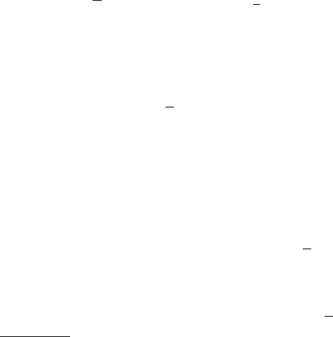
Fig. 3. Remarkable inequalities for propagation in a binary mixture of extinctions,

before correlations are considered. (a) The actual FPD is compared with its two

exponential components for σ

=0.2 and σ

=1.8withf

= f

=1/2 in (60);

the short steps are dominated by the dense half and the long ones be the tenuous

half. Two exponential approximations based on σ = f

+ f

= 1 and on the

actual MFP 1/σ = f

/σ

=2.77

...

are also plotted. (b) The actual MFP is

compared to the prediction 1/σ based on mean extinction as σ

/σ

increases from

1 to 10 and as the mixing ratio f

varies; the special case used in panels (a) and

) of the actual FPD are compared

with the exponential prediction Γ (q+1)1/σ

based on the actual MFP. The under-

estimation of moments at both higher-order (q>1) and negative order (q<0) is a

direct consequence of the wider-than-exponential nature of the actual FPD. Note

that, although their plotted ratio is ﬁnite, both moments are in fact divergent for

q ≤−1. Adapted from Fig. 1 in [27]

104 A.B. Davis

on s over a signiﬁcant range of s-values starting of course at 0. As it turns

out, this mandates that the extinction ﬁeld has correlations over that same

range of scales, at least in its 2-point statistics such as the (2nd-order) struc-

ture function, [σ(x + r) − σ(x)]

 where r, is a given displacement vector.

See the appendix in Davis and Marshak [27], with A. Benassi, for a detailed

proof.

This is just a formal way of making a quite natural assumption, one that

all instrument designers make to some extent for the purposes of signal-

to-noise management. We are simply saying that a (less noisy) estimate of

a spatial average is almost as good as a quasi-point-wise value, only with

some tolerable (and maybe correctable) loss of extreme values. And this in

turn requires that the optical medium has correlations over the range of

scales for which (74) applies. As shown by Davis and Marshak, the well-

documented turbulent/fractal structure of terrestrial clouds guarantees that

such correlations exist. Indeed, clouds are “scaling” in the sense that

|σ(x + r) −σ(x)|

∼r

ζ(p)

(75)

over a signiﬁcant range of scales r (2 to 3 orders of magnitude at least).

The l.-h. side of (75) is called the “pth-order structure function” and ζ(p)is

known to be a continuous concave function as long as the dependance on p

of the prefactors on the r.-h. side can be neglected (yet another consequence

of Jensen’s inequality). The exponents ζ(p) can in fact be obtained from the

spatial/ensemble statistics of h(x) in (74), and vice-versa, using Frisch and

Parisi’s [29] multifractal formalism. This kind of scaling is associated with

long-range correlations and leads to a correspondingly weak dependence on

s of the PDF of

in (72); see Fig. 4 for computations based on synthetic

turbulence data.

That is not the end of the story. It is important to assess the resilience

or fragility of Beer’s exponential transmission law to perturbation by 3D

variability. Under what conditions is the MFP signiﬁcantly larger than 1/σ?

Andwhenaretheqth-order moments (q>1) of s signiﬁcantly larger than

the prediction of the exponential distribution? Intuitively, this calls for two

conditions:

1. that the amplitude of the 1-point variability is suﬃcient (cf. Fig. 3b);

2. that at least some of the scales of correlated 2-point variability are com-

mensurate with the MFP.

In item 2, we are thinking about the actual MFP and not the biased estimate

1/σ. Recall that the actual MFP can become much larger than 1/σ if there

are signiﬁcant regions of low extinction (consider Fig. 3b when σ

becomes

very small).

Davis and Marshak call condition #2 “resonant” variability noting that

it is a rather broad resonance, easily achieved in terrestrial clouds and cloud

systems. So non-exponential transmission laws are expected to be the rule

Eﬀective Propagation Kernels in Structured Media 105

0.0

0.5

1.0

1.5

2.0

2.5

0 1000 2000 3000 4000 5000 6000 7000 8000

(x)

(a)

Log-normal variability model

0.001

0.01

0.1

0 0.5 1 1.5 2 2.5 3

PDF estimates

(normalized histgram for 10 realizations)

(x)

log

mode

median

mean±sigma

(b)

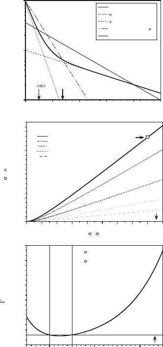
Fig. 4. Example of a transect through a random multifractal extinction ﬁeld with

lognormal statistics. This data is synthetic but the 1- and 2-point statistics are

typical of in-cloud extinction variability [30] and such stochastic models are used

routinely in 3D RT cloud studies. (a) Sample realization σ(x) with a log-normal

PDF generated by exponentiating fractional Brownian motion [31] with a wavenum-

ber spectrum in k

−5/3

; the mean (solid line) is set to unity and the std. dev. is ±1/3

(dashed lines). (b) Illustration of the “1-point scale-independence” property [27]:

PDFs of segment averages

(x) in (72) do not depend on segment length for all

but the most extreme values. Adapted from Fig. 6 in [27]

rather than the exception. Other situations can however arise, at least in the-

ory. At a given amplitude, even quite large amplitude variability can be “too

fast” or “too slow” to generate the interesting non-exponential transmission

laws. To wit,

• if the extinction ﬁeld is varying so fast that every photon can sample

essentially all the variability between almost every scattering, emission or

absorption event, then surely only the ensemble-mean extinction really

matters because that is (to high accuracy) the outcome of (72);

• in contrast, if the extinction ﬁeld varies so slowly that from its creation

to its absorption, escape or detection each photon samples basically just

one value of σ, then the ensemble-average transmission law is irrelevant

to the transport.

The former is the too-fast scenario, a.k.a. the atomistic mix (in stochastic RT

theory), and the pertinent approach to assess the bulk transport is to use the

mean properties in a homogeneous computation. The latter is the too-slow

scenario and an average over homogeneous multiple-scattering computations

weighted by the 1-point statistics of the extinction ﬁeld. This procedure is

known in cloud radiation studies as the Independent Pixel/Column Approx-

imation [8, 33].

106 A.B. Davis

Non-Poissonian Point-Process Approach

In this subsection, I adopt Kostinski’s [26] perspective on extinction as a

point process. I’ll start with uniform optical media. Inﬁnitesimal particles

are distributed at random, uniformly in space, according to some density n.

The photons in a given light beam interact with these particles simply where

they are, so extinction events

1. are a statistically homogeneous process, i.e., which does not depend on

position;

2. for small enough volumes, the probability of intercepting more than one

photon is vanishingly small; and

3. events in non-overlapping volumes are statistically independent.

These properties deﬁne a Poisson point-process [34]. So the discrete proba-

bility of obtaining exactly N ≥ 0 photon interactions (extinction events) over

a given distance s is

(s; m)=p

(m)=

× e

−m

(76)

where the sole parameter is the mean of N at given s,

m = E(N|s) . (77)

The variance D(N|s), deﬁned as in (56), of a Poisson deviate is equal to

its mean.

We also re-emphasize that, since we are averaging here over the

photon transfer events, we use the notation with E(·)’s.

Now, setting N = 0 (no events whatsoever over the segment of given

length s), we get p

(s)=exp(−m). By deﬁnition, this is direct transmission

dir

(s). We can therefore make the identiﬁcation

m = τ (s)=σs (78)

in (43), recalling that we found σ (in this case constant) to be particle density

n times the collision cross-section per particle s. This is reminiscent of the

interpretation of optical distance τ(s) as distance s in units of MFPs; more

precisely here, τ(s) is the average number of collisions m suﬀered over distance

s, at the average rate of one per MFP. Of course, at the single photon level,

only one such interaction is enough to remove it from the beam, however, a

small number of lucky ones can travel across large (optical) distances, that

is, several MFPs.

We now turn to “lumpiness” in non-uniform optical media, translating

to spatial correlations between the particles, hence between the extinction

This might sound dissonant to some readers on dimensional grounds. (Should

that not be standard deviation =

√

D? That is until we recall that this random

variable is a pure number: we are just counting events.

Eﬀective Propagation Kernels in Structured Media 107

events. In point process theory, correlation is deﬁned as the deviation from

Poissonian behavior in the joint probability of ﬁnding exactly one particle in

each of two small volumes δV

and δV

at a distance r:

Pr{N

= N

=1;n, r} = n

δV

[1 + η(r)] (79)

where n is the mean density of the particles. Because of their independence

in a uniformly random medium, the Poissonian prediction is η(r) = 0 while

η(r) = 0 corresponds to some kind of particle correlation in the medium. In

short, we retain above properties #1 and #2 but relax #3.

Another, more practical, way of deﬁning η(r) uses the “pair correlation”

N(0)N(r).Wehave

η(r)=N(0)N(r)/N 

− 1 (80)

where N is the number of particles in the small

test volume δV .Wehave

N = nδV and we consider two such volumes at a distance r. If the events

N(0) and N(r) are independent, then N(0)N(r) = N(0)N(r) = N

hence η(r) = 0. Note that, as in (61), we are averaging here over the disorder

of the particle distribution, hence the use of ·’s.

Following Landau and Lifschitz’s [35] general analysis of ﬂuctuations and

correlations in gases and liquids near a phase transition, it can be shown that,

in a small test volume δV , one has

δN

 = N  + ηN

(81)

where δN = N −N and

η is the volume average of η(r)overδV .For

example, we have

η(r)=



2

η(r



)dr



(82)

with r =

3δV/4π in the case of a spherical volume. Any deviation of η

from 0 in (81) takes event variance δN

 away from the Poissonian value of

N.

Returning to photon transport through a particulate medium, how do we

now estimate p

(s) in the presence of spatial correlations? For simplicity,

Kostinski proposes to use Mandel’s formula from statistical optics [36]:

p

(s) =

∞



(s|m)Pr(dm)=

∞



−m

Pr(dm) (83)

where Pr(dm) is the element of probability that the sole parameter of the

(discrete) Poissonian distribution in (76), now a (continuous) random vari-

able, falls between m and m +dm. Accordingly, we have transmuted the “;”

separator into a “|” in the argument of p

under the ﬁrst integral.

As nδV becomes small, we have N =0, 1 depending on whether a particle is

present or not, the former becoming the dominant event as soon as nδV  1.

108 A.B. Davis

For N = 0, this is equivalent to the computation of e

−τ(s)

 =



exp(−τ)

Pr(dτ|s) in (66) since τ is also equal to m = σs, σ being the random quantity

at present. So the three general properties of e

−τ(s)

 and its derived quan-

tities stated in Sect. 3.4 will follow from this alternative model for photon

transport.

The close formal analogy between (66) and (83) is traceable to the close

connection between collision statistics, (direct) transmission, and FPDs. The

essential diﬀerence between the continuum transport-theoretical and random

point-process approaches is that, coming from the latter less-familiar perspec-

tive, the question of spatial correlations (i.e., droplet clumping tendencies)

arises immediately, at any rate, before the question of how to average over

the spatial disorder. In the more familiar continuum approach, we ﬁrst ar-

gued for averaging the (partial) kernel and then argued that the outcome, as

strikingly diﬀerent as it is from an exponential, is only relevant if the optical

medium has spatial correlations that overlap with the MFP. The central role

of the MFP is not that obvious in the point-process framework.

3.5 Results for Gamma-Distributed Extinctions,

and Point-Process Equivalents

We assume here a Gamma-distribution for τ = m in (83) or, equivalently, for

τ = σs in (64) at a given distance s. The two parameters of this distribution

are the mean, σs,and

a =

τ(s)

(τ(s) −τ(s))





σ

/(σ −σ)

 in the continuum approach

m

/(m −m)

 in the point-process approach

(84)

where we recognize a variance in the denominator. So the degenerate (uniform

extinction, Poissonian events) case is retrieved in the limit a →∞: as in (59),

no variance at all. The PDF for τ(s), hence for m,readsas

Pr(dτ|s)=p(τ; σs, a)dτ =

Γ (a)



σs



×τ

a−1

exp[−aτ/σs]dτ.(85)

The second argument —and ﬁrst parameter— is the mean of τ(s). By writing

it as σs the given step size s appears. The Gamma-distribution has the

exponential (or Laplace) law of extinction variability as a special case when

a =1:

Pr(dτ|s)=p(τ; σs, 1)dτ =exp[−τ/σs]dτ/σs, (86)

not to be confused with (Beer’s) exponential law of direct transmission. As

another example, reconsider Figs. 4 where we see a synthetic in-cloud vari-

ability with a = 9 in (84), a reasonable amount of skewness (log-normal

a is the squared inverse of the standard non-dimensional variability parameter,

i.e., std.-dev./mean.

Eﬀective Propagation Kernels in Structured Media 109

PDF), and realistic 2-point correlations (associated with the prescribed k

−5/3

wavenumber spectrum).

In the continuum approach from Sect. 3.4, this choice of variability model

applied to (66) yields

T

dir

(s; σ,a)=e

−τ(s)

 =

(1 + σs/a)

(87)

for the mean transmission law which is plotted in Fig. 6b. As expected,

the exponential law exp(−σs) is recovered (using L’Hˆopital’s rule) in the

degenerate-σ limit a →∞. Otherwise, direct transmission is eﬀectively

power-law, with diverging moments E(s

) for q ≥ a. Assuming a>1,

the MFP exists and is given by

E(s) = σ

−1

 =



a − 1



σ

−1

. (88)

Notice the excess over the standard prediction using σ

−1

.Itiseasytoverify

here the general result that E(s) = 1/σ using the PDF in (85).

In the discrete point-process approach from Sect. 3.4, the same choice of

variability in (85) now reads as

Pr(dm|s)=p(m; σs, a)dm =

Γ (a)



σs



× m

a−1

exp[−am/σs]dm

(89)

where σs = m. Applying this to (83) leads to a so-called negative binomial

distribution for N. More precisely, we have

p

(s) = p

(σs, a)=

(σs)

Γ (N + a)

Γ (a)(a + σs)

(1 + σs/a)

. (90)

The case a ∈ N −{0} = {1, 2,...} is known as the Pascal distribution and

it arises naturally from the theory of Bernoulli processes. Speciﬁcally, the

question is about the probability of having exactly a ≥ 1 successes with

probability p and N ≥ 0 failures with probability q =1− p, ending with a

The above choice of variability model for τ(s) is not arbitrary. We have

adopted the convenient as well as reasonably accurate parameterization by

Barker et al. [37] of the observed variability of optical depth (measured ver-

tically) in high-resolution satellite images of a wide variety of cloud scenes.

Figure 5 reproduces their evidence for Gamma-distributions for τ (s), where

s is the thickness of the cloud layer using LandSat imagery with ≈30 m pix-

els and ≈60 km swaths. We note that Barker et al.’s determination of cloud

optical depth for each LandSat pixel is based, as usual in cloud remote sens-

ing, on a 1D RT model and this procedure is known to underestimate the

variance [38]; so the inferred values of a are likely to be upper bounds.