Graziani F. (editor) Computational Methods in Transport

Подождите немного. Документ загружается.

Parallel Solution of the Time-Dependent S

Equations 471

c∆t

n+1

+ Ω ·∇I

n+1

+ κ

(ε)I

n+1

−



dΩ





dε



n+1

(Ω



,ε



,Ω,ε)



S(ε)+

∆t



(2)

where we have suppressed the arguments of I in the integral term for clarity

and where we use standard ﬁnite-diﬀerence notation of superscripts to denote

the time at which the time-discretized analog of I is deﬁned:

≡ I(x,Ω,ε,t

) . (3)

We now consider the angular discretization of (2). For the sake of brevity

we restrict ourselves to 1-D geometries such as Cartesian or spherical coor-

dinates where the direction can be characterized by a single angle cosine µ

and (2) simpliﬁes to

c∆t

n+1

+ µ ·∇I

n+1

+ κ

(ε)I

n+1

− 2π



dµ





dε



n+1

(µ



,ε



,µ,ε)



S(ε)+

∆t



. (4)

Angular discretization in multi-dimensions is straightforward and the reader

is referred to [LM93] for details. In the discrete ordinates method the con-

tinuous range of the angular cosine, −1 ≤ µ ≤ 1, is replaced by a discrete

set of angular ordinates {µ

| k =1,...,N} for which (4) holds true. For

the direction µ

the angular integral in (4) is approximated by a compatible

quadrature



dµ



n+1

(µ



,ε



,µ,ε) ≈



=1



n+1



k,

(ε



,ε)(5)

where k and  are subscripts denoting directions µ

and µ



. The energy

integral can be dealt with similarly by discretizing the spectrum into a series

of groups with energies at the group center given by {ε

| g =1,...,M}

and the group widths given by {∆ε

| g =1,...,M}. For an energy ε

and

direction µ

the double integral in (4) is approximated by



dµ





dε



n+1

(µ



,ε



,µ,ε) ≈



=1



g=1

∆ε



n+1



k,h,,g

(6)

and the discrete analog of (4) becomes

c∆t

n+1

h,k

+ µ

·∇I

n+1

h,k

+ κ

n+1

h,k

− 2π



=1



g=1

∆ε



n+1



k,h,,g



h,k

∆t



. (7)

472 F.D. Swesty

Equation (7) is referred to as the S

equation or the monochromatic, discrete-

ordinates, Boltzmann equation.

In order to numerically solve (7) some form of spatial discretization is

applied to the streaming operator µ

·∇. This discretization may require some

sort of closure relationship relating the intensities at adjacent spatial points.

For a detailed description of a variety of spatial discretizations we refer the

reader to [PA92]. For any spatial discretization scheme that is linear in I

n+1

h,k

the set of equations (7) for all spatial zones, together with any linear equations

describing boundary conditions on the computational domain, forms a large,

sparse, linear system of equations that must be solved in order to obtain I

n+1

h,k

at each timestep.

3 Iterative Approaches

The linear systems described in Sect. 2 are sparse and, for multidimensional

problems, extremely large. The sparsity suggests the use of iterative methods

to solve the linear system. Direct solution methods for these linear systems

have been applied in one dimensional problems, e.g. [MB93], but in multi-

dimensional problems the size of the linear systems renders direct solution

methods impractical in most situations.

The iterative methods utilized have fallen into two categories. The ﬁrst are

source iteration methods, which split the linear systems into parts, solving

a portion of the system directly. This method has been widely utilized by

the neutronics community for many years [LM93]. The second approach has

been the use of Krylov subspace algorithms applied to the full linear system.

This method has seen only limited use in both the astrophysical community

[DM05] and the neutronics community [PH02].

3.1 Source Iteration

In this section we will brieﬂy describe the source iteration method in a linear

algebraic context. An alternative, and perhaps more physical, description is

provided in [LM93]. The linear system arising from the S

equations can be

written in the form of

Ax = b (8)

where x is a vector containing the unknowns I

n+1

h,k

and b is a vector made up

of the right-hand-sides of (7). The full linear system matrix A can be split

into parts arising from the various operators composing the left-hand-side of

(7)

A = D + T + S. (9)

In (9) D is a matrix arising from the time derivative and total opacity terms

on the left-hand-side of (7) and S is matrix arising from the scattering term.

The matrix T arises from the spatial discretization of the streaming operator.

Parallel Solution of the Time-Dependent S

Equations 473

In a 1-D problem, with a lexicographic ordering of variables, these matrices

may take on a very simple form where D may be diagonal or banded, T may

be tridiagonal, and S could consist of blocks of size NM × NM located on,

or adjacent to, the diagonal. In the general case D, T ,andS may be more

complex in structure.

The strategy behind the source iteration scheme is to exploit the splitting

to form an iterative scheme as follows:

1. An initial guess is made for the solution vector x

2. The equation

(D + T )x



= b − Sx (10)

is solved for x



using direct methods applied to the matrix D + T which

is usually banded for simple geometries and meshes.

3. set x = x



and repeat the procedure starting at step 1 until convergence

is obtained.

This simplistic iterative algorithm suﬀers from two major limitations that

run counter to the desiderata listed in Sect. 2.

The ﬁrst problem arises from the direct solve in step 2 of the source itera-

tion algorithm. This solve usually exploits the banded structure arising from

simple linear discretizations of the T operator by performing Gaussian elim-

ination via forward and back substitution steps. A physical interpretation

of this process is that one is sweeping in through the mesh in the direction

of radiation travel updating the intensity in the downwind direction. How-

ever, this approach is recursive and is not well suited to parallelization. In

simple Cartesian geometries with suﬃciently simple boundary conditions one

can exploit wave-front parallelization techniques [KBA92] to implement this

method on parallel architectures. However, complex boundary conditions and

curvilinear geometries couple equations with diﬀering values of the angular

cosines in a manner that makes such parallelization techniques diﬃcult.

The second problem with source iteration is that the method converges

poorly, or often fails to converge entirely, when the problems are scattering

dominated. The reason for this is obvious from (10) where the dominant

operator S is continually applied to the previous iterate on the right-hand-

side. This problem is not insurmountable in many cases and the convergence

can be hastened or obtained via the use of accelerators which provide better

initial guesses for step 1 of the source iteration algorithm.

There are two major beneﬁts to this algorithm in some circumstances.

First, in optically thin situations where there is little or no scattering the

solution of (10) provides a highly accurate in answer in very few iterations.

The second beneﬁt is that the algorithm requires little in the way of storage

especially if the scattering matrix can be applied in operator form or if it is

trivial as in the case of isotropic scattering.

474 F.D. Swesty

3.2 Full Linear System Solution via Krylov Subspace Iteration

An alternative approach to solving the linear systems arising from the S

equations is applying state-of-the-art Krylov subspace algorithms to obtain

the solution of the full linear system (8). The derivations of, and a description

of the features and limitations of various Krylov subspace algorithms are be-

yond the scope of this paper and the interested reader should consult [SA03]

or [BA94] for details. However, we will brieﬂy describe aspects of the algo-

rithms that are relevant to their use in solving the linear systems arising from

the S

equations.

There are several advantages to using nonstationary Krylov subspace al-

gorithms for nonsymmetric problems such as GMRES [SS86] or Bi-CGSTAB

[VO92] on the full linear system Ax = b:

• Algorithms can be implemented in operator, or matrix-free, form where

storage of the coeﬃcient matrix A is not required. The matrix-vector

multiply operation required by these algorithms can be implemented by

supplying a subprogram that evaluates the left-hand-side of the S

equa-

tion.

• Curvilinear coordinate systems or complex boundary conditions are rela-

tively easy to accommodate.

• Parallelism derives from the parallel nature of the sparse linear algebraic

operations involved in the Krylov subspace algorithm.

• Algorithms require only a few basic linear algebraic operations which

can usually be encoded using BLAS (Basic Linear Algebra Subprograms)

operations or their equivalents. Some of these operations such as vector

additions are embarrassingly parallel. Under a spatial domain decompo-

sition scheme the matrix-vector multiplies require only nearest-neighbor

communication within a process topology. Vector inner products can be

accomplished via global reduction operations supplied by the message

passing interface (MPI).

There are also drawbacks associated with the use of nonstationary Krylov

subspace algorithms. These algorithms require the use of temporary vectors

to hold intermediate results. Each of these vectors are identical in size to

the vector of unknowns x. Typically this means that the algorithms may re-

quire, at a minimum, 5–8 vectors worth of memory in addition to the memory

associated with the vector of unknowns. Some algorithms such as GMRES

require a number of vectors that grows as the iteration process progresses.

This growth in memory utilization can be mitigated in some cases by restart-

ing the iteration process anew (see [BA94] for details). For this reason we

restrict ourselves to discussing the Bi-CGSTAB algorithm for the remainder

of this paper.

Another drawback that nonstationary Krylov subspace algorithms share

with the source iteration process is that of non-convergence or slow

Parallel Solution of the Time-Dependent S

Equations 475

convergence in some circumstances. We brieﬂy examine these issues in the

next section.

4 Speeding Up and Obtaining Convergence

There are techniques to improve the iterative convergence of both the source

iteration method and the full linear system solution method. Since our focus

for the remainder of this paper is on the use of the full linear system solution

method we will only brieﬂy discuss techniques for improving the convergence

of source iteration. In the case of the full linear system solution we will

discuss one class of preconditioners that holds promise for use on parallel

architectures.

4.1 Accelerators

In the context of the source iteration approach improvements to iterative con-

vergence are usually sought by means of accelerators which provide a better

estimate for the vector of unknowns x for insertion into the right-hand-side

of (10) on each iterative step. The calculation of this estimate is achieved

via some algorithm that is usually referred to as an accelerator. There is

an entire body of literature on the development of accelerators. Readers are

urged to consult the excellent review article [AL02] for details. We conﬁne

ourselves here to a brief discussion of one broadly utilized class of accelera-

tors referred to as diﬀusion synthetic acceleration (DSA) techniques [AL77].

In these methods a discretized diﬀusion equation that is consistent with the

equation is solved for the energy density which is then used to evaluate

the scattering term on the right-hand-side of (10). This process accelerates

the convergence of source iteration in optically thick or optically translu-

cent situations. DSA schemes are usually derived for the case of isotropic

scattering but the can be extended to the anisotropic case as well [MO82].

Another challenge to the construction of eﬀective accelerators is that it is

often diﬃcult to construct a discretized diﬀusion equation that is consistent

with the S

equation. Larsen [LA82] has developed a four-step process for

constructing DSA accelerators but the construction can be complex for many

schemes [PA92].

4.2 Preconditioners

The convergence of the full linear system solution can be improved through

the use of preconditioners. The idea behind preconditioning is deceptively

simple. A dominant factor in the convergence of a nonstationary Krylov sub-

space algorithm is the condition number of the coeﬃcient matrix A. Precon-

ditioning seeks to improve the conditioning of the system by solving

476 F.D. Swesty

−1

x = M

b (11)

instead of solving (8). The matrices M

and M

are referred to as left and

right preconditioners respectively. A clever choice of preconditioners may

provide a coeﬃcient matrix M

−1

that has a better condition number

than does A.

As with accelerators there exists a vast body of literature on precon-

ditioners which is well beyond the scope of this paper. A recent review

by Benzi [BE02] provides a fairly comprehensive bibliography for this sub-

ject. The desire for parallel scalability restricts the choice of precondition-

ers to those that are parallelizable. Many traditional preconditioning tech-

niques that are used with Krylov subspace methods are inherently sequential.

Nevertheless these preconditioning techniques can at times be utilized suc-

cessfully in a parallel context [DM05].

Development of inherently parallel preconditioners is on ongoing area of

research. For this reason we will only brieﬂy mention one particular class

of preconditioners, sparse parallel approximate inverses (SPAI) which have

desirable scalability properties. SPAI preconditioners have been utilized suc-

cessfully on a variety of problems including radiation transport in the ﬂux-

limited diﬀusion approximation [SS04]. The idea behind SPAI preconditioners

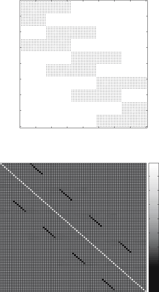
is quite simple. One wishes to exploit the sparsity pattern and the structure

of the coeﬃcient matrix to ﬁnd an eﬀective approximation to the inverse that

is sparse. The sparsity pattern of an example system arising from the dia-

mond diﬀerence spatial closure is shown in Fig. 1 which depicts an 80 × 80

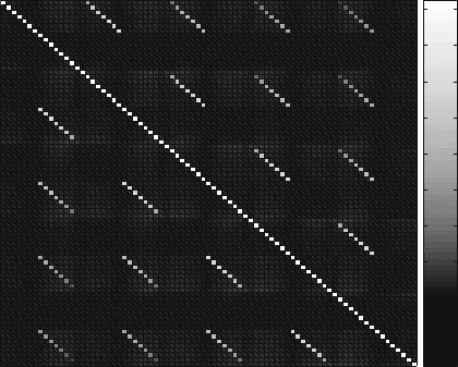
section of the upper left corner of the coeﬃcient matrix A. The values of the

elements in this matrix section are shown as a grayscale map in Fig. 2. The

coeﬃcient matrix A has been row scaled so that the diagonal elements have

a value of unity. Figure 2 clearly shows that dominant oﬀ-diagonal elements

lie in bands spaced a distance equal to the number of ordinates (N =16in

this case) away from the diagonal.

A pattern is chosen for the non-zero elements in the approximate inverse.

The choice of pattern may or may not be inﬂuenced by the values of the

elements in the true inverse A

−1

. Ideally we would like to ﬁnd a left or right

approximate inverse by choosing values for the non-zero elements such that

≈ A

−1

or M

−1

≈ A

−1

. The values of the non-zero elements are in

general over-determined but we can ﬁnd an optimal set of values by doing a

least squares ﬁt to determine the values of the non-zero elements in each row

of M

or column of M

−1

. For details of this procedure consult [BE02] and

references therein. The inverse A

−1

may have structure that can be exploited

in forming the sparse approximate inverse. An example of this is illustrated in

Fig. 3 where the grayscale image shows the value of each element of the upper-

left 80×80 corner of the inverse of the matrix shown in Fig. 2. One can clearly

see that the dominant elements of the inverse lie along the diagonal and in

bands that are spaced a distance equal to integer multiples of the number of

angular ordinates away from the diagonal. This inverse structure is typical for

Parallel Solution of the Time-Dependent S

Equations 477

0 10 20 30 40 50 60 70 80

Fig. 1. A diagram of the sparsity pattern of the coeﬃcient matrix A arising from

the diamond diﬀerenced S

equations for N =16

706050403020100

−0.8

−0.6

−0.4

−0.2

0.2

0.4

0.6

0.8

Fig. 2. A grayscale map of the elements in the upper left 80 × 80 corner of the

coeﬃcient matrix A arising from the diamond diﬀerenced S

equations for N =16

478 F.D. Swesty

706050403020100

0.1

0.2

0.3

0.4

0.5

0.6

0.7

0.8

0.9

Fig. 3. A grayscale map of the elements in the upper left 80 × 80 corner of the

inverse coeﬃcient matrix A

−1

arising from the diamond diﬀerenced S

equations

for N =16

the inverse of matrices arising from partial diﬀerential equations with local

spatial coupling [SM05]. The size of the oﬀ-diagonal elements decays slightly

as one moves away from the diagonal.

The time dependence of the Boltzmann equation also factors into struc-

ture of the inverse. In simulations where the time evolution is being carried

out with small CFL number timesteps the D matrix will dominate the coeﬃ-

cient matrix A. In this case the system is likely to be diagonally dominant. In

the case of diagonal dominance of a matrix that can be formulated in a block

tridiagonal form the inverse has elements that decay in size exponentially as

one moves away from the diagonal (see [AX96] Sect. 8.6 for details ). Such a

situation is ideal for approximate inverse preconditioners since the inverse can

be eﬀectively approximated with only a few bands. If the timestep sizes are

increased eventually the behavior of the S

equation becomes more elliptic

and the decay behavior in the inverse becomes less pronounced. In the inverse

depicted in Fig. 3 the decay of the elements is slight as there is no time de-

pendence in this problem. However, even in the large CFL number timestep

limit simple SPAI preconditioners can continue to preform remarkably well.

A major advantage of the procedure for forming the SPAI preconditioner

is that under a spatial domain decomposition the least squares ﬁt of each

row or column of the preconditioner can be performed in parallel with only

nearest-neighbor communication if the sparsity pattern involves elements cor-

responding to only nearby spatial zones. In general for the S

equation this

is true as the spatial discretization usually couples only a few neighboring

zones. This localized structure of the linear system can thus be exploited to

yield fairly eﬀective parallel preconditioners for the S

equation.

Parallel Solution of the Time-Dependent S

Equations 479

4.3 A Brief Comparison of Approaches

In this section we oﬀer a brief comparison of the source iteration and full

linear system solution approaches on a series of 1-D test problems with and

without reﬂective boundaries that illustrate a few of the points mentioned

in Sects. 4.1 and 4.3. For the sake of simplicity we consider the diamond-

diﬀerence scheme in Cartesian or slab geometry. The details of the source

iteration method and the DSA accelerator for this case are fully documented

in [AL77].

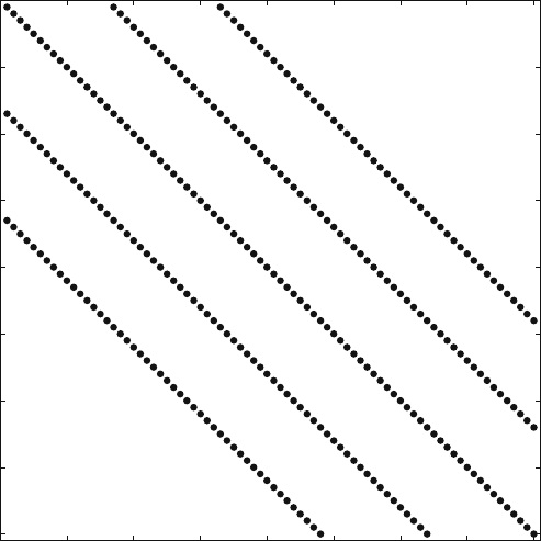
The full linear system solution is accomplished with the Bi-CGSTAB

algorithm. We consider a SPAI preconditioner with ﬁve non-zero elements

per row. The sparsity pattern for this preconditioner is shown in Fig. 4 where

we show the upper-left 80 × 80 corner of A

−1

. This preconditioner is easily

implemented and the values of the elements need only be computed once and

stored in an array. The storage cost of the vector is approximately the cost

of 5 unknown vectors.

The ﬁrst problem we consider is a 1-D translucent slab with incoming

boundary conditions on either end. The problems is zoned into 1024 uniform

0 30

0 50 60

0 80

Fig. 4. A diagram of the sparsity pattern of the approximate inverse preconditioner

used in the comparison for N = 16. The spacing between the bands is equal to the

number of quadrature points

480 F.D. Swesty

500

1000

1500

2000

2500

3000

3500

0 5 10 15 20 25 30

Iterations

Number of Quadrature Points

500

1000

1500

2000

2500

3000

3500

0 5 10 15 20 25 30

Iterations

Number of Quadrature Points

500

1000

1500

2000

2500

3000

3500

0 5 10 15 20 25 30

Iterations

Number of Quadrature Points

500

1000

1500

2000

2500

3000

3500

0 5 10 15 20 25 30

Iterations

Number of Quadrature Points

500

1000

1500

2000

2500

3000

3500

0 5 10 15 20 25 30

Iterations

Number of Quadrature Points

500

1000

1500

2000

2500

3000

3500

0 5 10 15 20 25 30

Iterations

Number of Quadrature Points

500

1000

1500

2000

2500

3000

3500

0 5 10 15 20 25 30

Iterations

Number of Quadrature Points

500

1000

1500

2000

2500

3000

3500

0 5 10 15 20 25 30

Iterations

Number of Quadrature Points

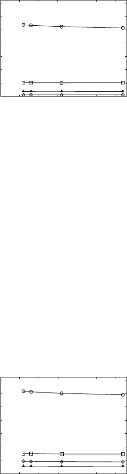
Fig. 5. Number of Iterations versus the number of angular quadrature points for the

slab geometry problem. Circles denote the unaccelerated source iteration method.

Squares denote the unpreconditioned Bi-CGSTAB method. Triangles indicate the

Bi-CGSTAB preconditioned with a simple SPAI preconditioner with 5 non-zero

elements per row. Diamonds indicate source iteration with DSA acceleration

width zones and the opacity is such that each zone has an optical depth of

0.1. There are no sources and no time-dependence in the problem.

The comparative performance of the source iteration and Bi-CGSTAB

applied to the full linear system are shown in Fig. 5. The unpreconditioned Bi-

CGSTAB converges in substantially fewer iterations than does the source iter-

ation method. However, with the addition of a DSA accelerator the source it-

eration method converges in far fewer iterations than the Bi-CGSTAB+SPAI

combination. Also, the behavior is clearly independent of the angular resolu-

tion.

The second problem is almost identical to the ﬁrst with the exception

that it has a reﬂective boundary on the right end of the computational do-

main. In this case results shown in Fig. 6 the Bi-CGSTAB+SPAI combination

proves superior converging in substantially fewer iterations than the source

iteration+DSA combination.

500

1000

1500

2000

2500

3000

3500

0 5 10 15 20 25 30

Iterations

Number of Quadrature Points

500

1000

1500

2000

2500

3000

3500

0 5 10 15 20 25 30

Iterations

Number of Quadrature Points

500

1000

1500

2000

2500

3000

3500

0 5 10 15 20 25 30

Iterations

Number of Quadrature Points

500

1000

1500

2000

2500

3000

3500

0 5 10 15 20 25 30

Iterations

Number of Quadrature Points

500

1000

1500

2000

2500

3000

3500

0 5 10 15 20 25 30

Iterations

Number of Quadrature Points

500

1000

1500

2000

2500

3000

3500

0 5 10 15 20 25 30

Iterations

Number of Quadrature Points

500

1000

1500

2000

2500

3000

3500

0 5 10 15 20 25 30

Iterations

Number of Quadrature Points

500

1000

1500

2000

2500

3000

3500

0 5 10 15 20 25 30

Iterations

Number of Quadrature Points

Fig. 6. Same as Fig. 5 but for the reﬂecting boundary problem