Greenwood D.T. Advanced Dynamics

Подождите немного. Документ загружается.

89 Hamilton’s equations

Now the generalized momentum p

∂T

∂

= mr



+ cos θ



θ (2.116)

and we obtain

θ =



+ cos θ



(2.117)

The kinetic energy as a function of (q, p)is

T =

2mr



+ cos θ



(2.118)

The potential energy is

V = mg



−rθ sin α +

r cos(θ + α)



(2.119)

The Hamiltonian function is, in general,

H = T

− T

+ V (2.120)

but, in this case, it is equal to the total energy.

H =

2mr



+ cos θ



+ mg



−rθ sin α +

r cos(θ + α)



(2.121)

The ﬁrst canonical equation results in

θ =

∂ H

∂p



+ cos θ



(2.122)

which is a restatement of (2.117). The second canonical equation is

=−

∂ H

∂θ

−p

sin θ

2mr



+ cos θ



+ mgr



sin α +

sin(θ + α)



(2.123)

These two canonical equations are together equivalent to the single second-order equation

in θ which would be obtained by using Lagrange’s equation.

Second method Let us use the same system to illustrate the use of Lagrange multipliers

with Hamilton’s equations, as in (2.111). We will use (x,θ) as generalized coordinates,

where x is the displacement of the center of the disk. There is a holonomic constraint

x −r

θ = 0 (2.124)

which expresses the nonslipping condition. The kinetic and potential energies, however,

must be written for the unconstrained system, that is, assuming the possibility of slipping.

The kinetic energy is

T =



θ cos θ



(2.125)

90 Lagrange’s and Hamilton’s equations

and the potential energy is

V = mg



−x sin α +

r cos(θ + α)



(2.126)

The generalized momenta are

∂T

∂

= m

x +

θ cos θ (2.127)

∂T

∂

x cos θ +

θ (2.128)

Equations (2.127) and (2.128) can be solved for

x and

θ. We obtain

x =

− 2 p

cos θ

mr sin

(2.129)

θ =

4 p

− 2rp

cos θ

sin

(2.130)

Substituting these expressions for

x and

θ into the kinetic energy equation, we obtain, after

some algebraic simpliﬁcation, the Hamiltonian function

H = T + V =

2mr

sin



+ 4 p

− 4rp

cos θ



+ V (2.131)

where V is given by (2.126).

We shall use Hamilton’s equations in the form

∂ H

∂p

=−

∂ H

∂q



j=1

(i = 1,...,n) (2.132)

where, from (2.124), the constraint coefﬁcients are

= 1, a

=−r (2.133)

The

x equation is

x =

∂ H

∂p

− 2 p

cos θ

mr sin

(2.134)

The

equation is

=−

∂ H

∂x

+ λ =−

∂V

∂x

+ λ = mg sin α + λ (2.135)

The

θ equation is

θ =

∂ H

∂p

4 p

− 2rp

cos θ

sin

(2.136)

91 Integrals of the motion

Finally, the

equation is

=−

∂ H

∂θ

−rλ

sin



+ 4 p



cos θ − 2rp

(1 +cos

θ)



mgr sin(θ + α) −rλ (2.137)

These four ﬁrst-order Hamiltonian equations plus the constraint equation (2.124) can be

integrated numerically to solve for the 2 qs, 2ps, and λ as functions of time.

For a scleronomic system such as the one we have been considering, relatively simple

matrix equations can be used to obtain the Hamiltonian function. The kinetic energy is

quadratic in the

qs and of the form

T =

q (2.138)

where m is the n × n matrix of generalized mass coefﬁcients. The generalized momenta

are given by the matrix equation

p = m

q (2.139)

and, conversely,

q = bp (2.140)

where b = m

−1

. For scleronomic systems, the Hamiltonian function is equal to the total

energy, or

H = T + V =

bp + V (2.141)

For the system of this example, we have

m =



mr cos θ



(2.142)

and

b =

sin



−

r cos θ

−

r cos θ 1



(2.143)

in agreement with (2.131) and (2.141).

2.3 Integrals of the motion

We have found that for a dynamical system whose conﬁguration is given by n indepen-

dent generalized coordinates, the Lagrangian method results in n second-order differential

92 Lagrange’s and Hamilton’s equations

equations of motion with time as the independent variable. Any general analytical solution

of these equations of motion contains 2n constants of integration which are usually evalu-

ated from the 2n initial conditions. One method of expressing the general solution is to ﬁnd

2n independent functions of the form

(q,

q, t) = α

( j = 1,...,2n) (2.144)

where the αs are constants. The 2n functions are called integrals or constants of the motion.

Each function g

maintains a constant value α

during the actual motion of the system. In

principle, these 2n equations can be solved for the qs and

qs as functions of the αs and t,

that is,

= q

(α, t)(i = 1,...,n) (2.145)

(α, t)(i = 1,...,n) (2.146)

where these solutions satisfy (2.144).

Usually it is not possible to obtain a full set of 2n integrals of the motion by any direct

process. Nevertheless, the presence of a few integrals such as those representing conservation

of energy or momentum are very useful in characterizing the motion of a system.

If one uses the Hamiltonian approach to the equations of motion, integrals of the motion

have the form

(q, p, t) = α

( j = 1,...,2n) (2.147)

Under the proper conditions, the Hamiltonian function itself can be an integral of the motion.

Conservative system

A common example of an integral of the motion is the energy integral E(q,

q, t) which is

quadratic in the

qs and is expressed in units of energy. It satisﬁes the equation

E(q,

q, t) = h (2.148)

where h is a constant that is normally evaluated from initial conditions. For scleronomic

systems with T = T

, the energy integral, if it exists, is equal to the sum of the kinetic and

potential energies. More generally, however, the energy integral is not equal to the total

energy. Usually it is not an explicit function of time.

Let us deﬁne a conservative system as a dynamical system for which an energy integral

can be found. To obtain sufﬁcient conditions for the existence of an energy integral, let us

consider a system which is described by the standard nonholonomic form of Lagrange’s

equation.



∂ L

∂



−

∂ L

∂q



j=1

(i = 1,...,n) (2.149)

This equation is valid for holonomic or nonholonomic systems whose applied forces are

derivable from a potential energy function V (q, t ).

93 Integrals of the motion

Multiply (2.149) by

and sum over i. The result is



i=1





∂ L

∂



−

∂ L

∂q





i=1



j=1

(2.150)

We note that



i=1



∂ L

∂







i=1

∂ L

∂



−



i=1

∂ L

∂

(2.151)

where





i=1

∂ L

∂



= 2

(2.152)

Furthermore,



i=1

∂ L

∂

L −



i=1

∂ L

∂q

−

∂ L

∂t

(2.153)

and

L =

−

V (2.154)

Hence, from (2.150)–(2.154), we obtain

−

V =



i=1



j=1

−

∂ L

∂t

(2.155)

If the right-hand side of (2.155) remains equal to zero as the motion proceeds, then

E = T

− T

+ V is an energy integral and the system is conservative. The ﬁrst term on the

right-hand side will be zero if the nonholonomic constraint equations of the form of (2.113)

have all a

= 0; that is; if they are all catastatic. The second term on the right-hand side

will be zero if neither T nor V is an explicit function of time.

To summarize, a system having holonomic or nonholonomic constraints will be conser-

vative if it meets the following conditions:

1. The standard form of Lagrange’s equation, as given by (2.149) applies.

2. All constraints can be written in the form



i=1

= 0(j = 1,...,m) (2.156)

that is, all a

= 0.

3. The Lagrangian function L = T − V is not an explicit function of time.

94 Lagrange’s and Hamilton’s equations

These are sufﬁcient conditions for a conservative system. For systems with independent

qs, Lagrange’s equation has the simpler form



∂ L

∂



−

∂ L

∂q

= 0(i = 1,...,n) (2.157)

If this equation applies, and if ∂ L/∂t = 0, then the system is conservative.

Now let us consider the Hamiltonian approach to conservative systems. Suppose that a

system can be described by Hamilton’s equations of the form

∂ H

∂p

=−

∂ H

∂q



j=1

(i = 1,...,n) (2.158)

The Hamiltonian function will be a constant of the motion if

H =



i=1

∂ H

∂q



i=1

∂ H

∂p

∂ H

∂t

= 0 (2.159)

Substituting from (2.158) into (2.159), we ﬁnd that

H =



i=1



j=1

∂ H

∂t

(2.160)

We see that the system will be conservative and H (q, p) will be a constant of the motion



i=1

= 0(j = 1,...,m) (2.161)

that is, if a

= 0 for all j, and if the Hamiltonian function is not an explicit function of

time, implying that

∂ H

∂t

= 0 (2.162)

These conditions are equivalent to those found earlier with the Lagrangian approach. Thus,

the energy integral is

H = T

− T

+ V = E (2.163)

Finally, it should be noted from the ﬁrst equality of (2.159) that if the canonical equations

(2.100) apply, then

H =

∂ H

∂t

(2.164)

whether the system is conservative or not.

Example 2.5 A particle of mass m can slide without friction on a rigid wire in the form

of a circle of radius r , as shown in Fig. 2.5. The circular wire rotates about a vertical axis

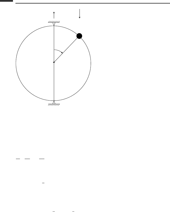
95 Integrals of the motion

Ω

Figure 2.5.

through the center O with a constant angular velocity . We wish to determine if this system

is conservative.

First, notice that this is a rheonomic holonomic system. It is possible, however, to choose

a single independent generalized coordinate θ. The system is described by Lagrange’s

equation of the form



∂ L

∂



−

∂ L

∂θ

= 0 (2.165)

as in (2.157). The Lagrangian function is

L = T − V =

m (r



sin

θ) −mgr cos θ (2.166)

which is not an explicit function of time. Hence, the sufﬁcient conditions for a conservative

system are met. The energy integral, which is constant during the motion is

E = T

− T

+ V =

−



sin

θ + mgr cos θ (2.167)

This, of course, is different from the total energy T + V .

It is interesting to study the same system using the Cartesian coordinates (x, y, z)to

specify the position of the particle. Let the Cartesian frame be ﬁxed in space with its origin

at the center O and with the positive z-axis pointing upward and lying on the axis of rotation.

Choose the time reference such that, at t = 0, the circular wire lies in the xz-plane. The

96 Lagrange’s and Hamilton’s equations

transformation equations are

x = r sin θ cos t (2.168)

y = r sin θ sin t (2.169)

z = r cos θ (2.170)

Notice the explicit functions of time, conﬁrming that the system is rheonomic.

The Lagrangian function has the simple form

L = T − V =

m (

) −mgz (2.171)

which is not an explicit function of time. There are two holonomic constraints, namely,

= x

+ y

+ z

−r

= 0 (2.172)

= x tan t − y = 0 (2.173)

Upon differentiation with respect to time, we obtain forms that are linear in the

qs, that is,

= 2

(

x + y

y + z

)

= 0 (2.174)

x tan t −

y + x sec

t = 0 (2.175)

The second constraint equation has a

= 0, so the sufﬁcient conditions for a conservative

system are not met with this Cartesian formulation. Here the energy function would equal

the total energy T + V , which is not constant because there is a nonzero driving moment

about the vertical axis.

Nevertheless, the energy function found earlier in (2.167) remains constant and is a valid

energy integral. When expressed in terms of Cartesian coordinates, it is

E =

m[(

x cos t +

y sin t)

] −

m

+ y

) +mgz (2.176)

We conclude that the system should be classed as conservative even though it does not meet

the sufﬁcient conditions in the Cartesian formulation.

Ignorable coordinates

Consider a holonomic system which is described by Hamilton’s canonical equations.

∂ H

∂p

=−

∂ H

∂q

(i = 1,...,n) (2.177)

Now suppose that the Hamiltonian function has the form

H(q

k+1

,...,q

, p

,..., p

, t), that is, the ﬁrst kqs do not appear. Then we ﬁnd that

=−

∂ H

∂q

= 0(i = 1,...,k) (2.178)

and therefore the ﬁrst k generalized momenta are

= β

(i = 1,...,k) (2.179)

97 Integrals of the motion

where the βs are constants. The kqs which do not appear in the Hamiltonian function are

called ignorable coordinates. The constant psareintegrals of the motion, in accordance

with (2.147).

The Hamiltonian function can now be written in the form

H(q

k+1

,...,q

, p

k+1

,..., p

,β

,...,β

, t). The canonical equations, assuming k ignor-

able coordinates, are

∂ H

∂p

=−

∂ H

∂q

(i = k + 1,...,n) (2.180)

Thus, k degrees of freedom corresponding to the k ignorable coordinates have been removed

from the equations of motion. The motion of the ignorable coordinates can be recovered by

integrating

∂ H

∂β

(i = 1,...,k) (2.181)

Now let us consider ignorable coordinates from the Lagrangian viewpoint. We assume a

holonomic system whose equations of motion have the standard Lagrangian form



∂ L

∂



−

∂ L

∂q

= 0(i = 1,...,n) (2.182)

First, recall from (2.97) that

∂ L

∂q

=−

∂ H

∂q

(i = 1,...,n) (2.183)

Hence, if a certain ignorable coordinate q

is missing from the Hamiltonian function, it will

also be missing from the Lagrangian function. If the ﬁrst kqs are ignorable, the Lagrangian L

will be a function of (q

k+1

,...,q

,...,

, t). We would like to eliminate the ignorable

qs from the Lagrangian formulation in order to reduce the number of degrees of freedom

in the equations of motion.

This goal may be accomplished by ﬁrst deﬁning a Routhian function R(q

k+1

,...,q

k+1

,...,

,β

,...,β

, t) as follows:

R = L −



i=1

(2.184)

where the ignorable

qs have been eliminated by solving the k equations

∂ L

∂

= β

(i = 1,...,k) (2.185)

for (

,...,

) in terms of (q

k+1

,...q

k+1

,...,

,β

,...,β

, t).

Now let us make an arbitrary variation in the Routhian function, including variations in

the βs and time. We obtain

δ R =



i=k+1

∂ R

∂q

δq



i=k+1

∂ R

∂



i=1

∂ R

∂β

δβ

∂ R

∂t

δt (2.186)

98 Lagrange’s and Hamilton’s equations

Next, take the variation of the right-hand side of (2.184). We have



L −



i=1





i=k+1

∂ L

∂q

δq



i=1

∂ L

∂



i=k+1

∂ L

∂

∂ L

∂t

δt

−



i=1

−



i=1

δβ

(2.187)

Using (2.185), this simpliﬁes to



L −



i=1





i=k+1

∂ L

∂q

δq



i=k+1

∂ L

∂

−



i=1

δβ

∂ L

∂t

δt (2.188)

We assume that the varied quantities in (2.186) and (2.188) are independent, and therefore

the corresponding coefﬁcients must be equal. Thus,

∂ L

∂q

∂ R

∂q

(i = k + 1,...,n) (2.189)

∂ L

∂

∂ R

∂

(i = k + 1,...,n) (2.190)

=−

∂ R

∂β

(i = 1,...,k) (2.191)

∂ L

∂t

∂ R

∂t

(2.192)

Now let us substitute from (2.189) and (2.190) into Lagrange’s equation, (2.182). We

obtain



∂ R

∂



−

∂ R

∂q

= 0(i = k + 1,...,n) (2.193)

These equations are of the form of Lagrange’s equation with the Routhian function replac-

ing the Lagrangian function. There are (n − k) second-order equations in the nonignorable

variables. Thus, the Routhian procedure has succeeded in eliminating the ignorable coor-

dinates from the equations of motion and, in effect, has reduced the number of degrees of

freedom to (n − k). Usually there is no need to solve for the ignorable coordinates, but, if

necessary, they can be recovered by integrating (2.191). The k integrals of the motion asso-

ciated with the ignorable coordinates are given by (2.185) and are equal to the corresponding

generalized momenta.

Example 2.6 Consider the same system as in Example 2.5 on page 94 (Fig. 2.5) except

that it can rotate freely about the ﬁxed vertical axis through the center, the angle of rotation

being φ. We ﬁnd that (φ,θ) are the generalized coordinates and the Lagrangian function is

L = T − V =

sin

θ +

− mgr cos θ (2.194)