Harris C.M., Piersol A.G. Harris Shock and vibration handbook

Подождите немного. Документ загружается.

Since f(x) is an odd function and noting that ωt varies from 0 to π/2 as x varies from

0 to A,

dζ







f(ξ) dξ

(4.23)

With ω

and φ

determined by Eqs. (4.23) and (4.22), respectively, the next

approximation may be found from the equation

x″+κ

f(x) − p cos φ

= 0 (4.24)

In the original differential equation, Eq. (4.20), ωt is replaced by its first approxima-

tion φ

and ω

(now known) is replaced by its second approximation ω

, thus giving

Eq. (4.24). This equation is again of a type which may be integrated explicitly; there-

fore, the next approximation ω

and φ

may be determined. In those cases where f(x)

is a complicated function, the integrals may be evaluated numerically.

This method involves reducing nonautonomous systems to autonomous ones* by

an iteration procedure in which the solution of the free vibration problem is used to

replace the time function in the original equation, which is then solved again for t(x).

The method is accurate and frequently two iterations will suffice.

THE PERTURBATION METHOD

In one of the most common methods of nonlinear vibration analysis, the desired

quantities are developed in powers of some parameter which is considered small;

then the coefficients of the resulting power series are determined in a stepwise man-

ner. The method is straightforward, although it becomes cumbersome for actual

computations if many terms in the perturbation series are required to achieve a

desired degree of accuracy.

Consider Duffing’s equation, Eq. (4.16), in the form

x″+κ

(x +µ

) − p cos φ=0 (4.25)

where φ=ωt and primes denote differentiation with respect to φ. The conditions at

time t = 0 are x(0) = A and x′(0) = 0, corresponding to harmonic solutions of period

2π/ω.Assume that µ

and p are small quantities, and define κ

 ε, p  εp

.The dis-

placement x(φ) and the frequency ω may now be expanded in terms of the small

quantity ε:

x(φ) = x

(φ) +εx

(φ) +ε

(φ) +

...

(4.26)

ω=ω

+εω

+ε

...

The initial conditions are taken as x

(0) = x

′(0) = 0 [i = 1,2,...].

Introducing Eq. (4.26) into Eq. (4.25) and collecting terms of zero order in ε gives

the linear differential equation

″+κ

= 0

2





κπ



NONLINEAR VIBRATION 4.25

* An autonomous system is one in which the time does not appear explicitly, while a nonautonomous sys-

tem is one in which the time does appear explicitly.

8434_Harris_04_b.qxd 09/20/2001 11:30 AM Page 4.25

Introducing the initial conditions into the solution of this linear equation gives

= A cos ωt and ω

=κ. Collecting terms of the first order in ε,

″+κ

− (2ω

A −

⁄4A

+ p

) cos φ+

⁄3A

cos 3φ=0 (4.27)

The solution of this differential equation has a nonharmonic term of the form φ cos φ,

but since only harmonic solutions are desired, the coefficient of this term is made to

vanish so that



⁄4A

−



Using this result and the appropriate initial conditions, the solution of Eq. (4.27) is

= (cos 3φ−cos φ)

To the first order in ε, the solution of Duffing’s equation, Eq. (4.25), is

x = A cos ωt +ε (cos 3ωt − cos ωt)

ω=κ+



⁄4A

−



This agrees with the results obtained previously [Eqs. (4.18) and (4.19)]. The analy-

sis may be carried beyond this point, if desired, by application of the same general

procedures.

As a further example of the perturbation method, consider the self-excited sys-

tem described by Van der Pol’s equation

¨x −ε(1 − x

)˙x +κ

x = 0 (4.5)

where the initial conditions are x(0) = 0, ˙x(0) = Aκ

. Assume that

x = x

+εx

+ε

...

=κ

+εκ

+ε

...

Inserting these series into Eq. (4.5) and equating coefficients of like terms, the result

to the order ε

x =



2 −



sin κ

t + cos κ

t +



sin 3κ

t − cos 3κ



− sin 5κ

(4.28)

THE METHOD OF KRYLOFF AND BOGOLIUBOFF

Consider the general autonomous differential equation

¨x + F(x,˙x) = 0

which can be rewritten in the form

¨x +κ

x +εf(x,˙x) = 0[ε << 1] (4.29)

5ε



124κ

3ε



4κ



4κ



4κ

29ε



96κ



2κ



32κ



32κ



2κ

4.26 CHAPTER FOUR

8434_Harris_04_b.qxd 09/20/2001 11:30 AM Page 4.26

For the corresponding linear problem (ε  0), the solution is

x = A sin (κt +θ) (4.30)

where A and θ are constants.

The procedure employed often is used in the theory of ordinary linear differen-

tial equations and is known variously as the method of variation of parameters or

the method of Lagrange. In the application of this procedure to a nonlinear equation

of the form of Eq. (4.29), assume the solution to be of the form of Eq. (4.30) but with

A and θ as time-dependent functions rather than constants. This procedure, how-

ever, introduces an excessive variability into the solution; consequently, an addi-

tional restriction may be introduced.The assumed solution, of the form of Eq. (4.30),

is differentiated once considering A and θ as time-dependent functions; this is made

equal to the corresponding relation from the linear theory (A and θ constant) so that

the additional restriction

A(t) sin [κt +θ(t)] +

θ(t)A(t) cos [κt +θ(t)] = 0 (4.31)

is placed on the solution. The second derivative of the assumed solution is now

formed and these relations are introduced into the differential equation, Eq. (4.29).

Combining this result with Eq. (4.31),

A(t) =−



f[A(t) sin Φ, A(t)κ cos Φ] cos Φ

θ(t) = f[A(t) sin Φ, A(t)κ cos Φ] sin Φ

where Φ=κt +θ(t)

Thus, the second-order differential equation, Eq. (4.29), has been transformed into

two first-order differential equations for A(t) and θ(t).

The expressions for

A(t) and

θ(t) may now be expanded in Fourier series:

A(t) =−



(A) +



n = 1

[Κ

(A) cos nΦ+L

(A) sin nΦ]



(4.32)

θ(t) =



(A) +



n = 1

(A) cos nΦ+Q

(A) sin nΦ]



where

(A) = 

2π

f[A sin Φ, Aκ cos Φ] cos Φ dΦ

(A) = 

2π

f[A sin Φ, Aκ cos Φ] sin Φ dΦ

It is apparent that A and θ are periodic functions of time of period 2π/κ; therefore,

during one cycle, the variation of

A and

θ is small because of the presence of the

small parameter ε in Eqs. (4.32). Hence, the average values of

A and

θ are consid-



2π



2π



κA



κA(t)



NONLINEAR VIBRATION 4.27

8434_Harris_04_b.qxd 09/20/2001 11:30 AM Page 4.27

ered. Since the motion is over a single cycle, and since the terms under the summa-

tion signs are of the same period and consequently vanish, then approximately:

A  −



(A)

θ  P

(A)

Φ  κ+ P

(A)

For example, consider Rayleigh’s equation

¨x − (α−β˙x

)˙x +κ

x = 0 (4.33)

By application of the above procedures:

A =−



(A) =−





2π

(−α + βA

cos

Φ)Aκ cos

Φ dΦ



= (α−

⁄4βA

) (4.34)

Equation (4.34) may be integrated directly:

t = 2



= ln

Solving for A,

A =



1 +



− 1



−αt



1/2

(4.35)

where γ=

⁄4β

(4.36)

The application of the method to Van der Pol’s equation, Eq. (4.5), is easily

accomplished and leads to a solution in the first approximation of the form similar

to that of the perturbation solution given by Eq. (4.28).

THE RITZ METHOD

In addition to methods of nonlinear vibration analysis stemming from the idea of

small nonlinearities and from extensions of methods applicable to linear equations,

other methods are based on such ideas as satisfying the equation at certain points of

the motion or satisfying the equation in the average. The Ritz method is an example

of the latter method and is quite powerful for general studies.

One method of determining such “average” solutions is to multiply the differential

equation by some “weight function” ψ

(t) and then integrate the product over a period

of the motion. If the differential equation is denoted by E, this procedure leads to



2π

E⋅ψ

(t) dt = 0 (4.37)



γA



α−γA





A(α−γA

)



2π



κA



κA



4.28 CHAPTER FOUR

8434_Harris_04_b.qxd 09/20/2001 11:30 AM Page 4.28

A second method of obtaining such average solutions can be derived from the

calculus of variations by seeking functions that minimize a certain integral:

I =



F(˙x,x,t) dt = minimum

Consider a function of the form

˜x(t) = a

(t) + a

(t) +

...

+ a

(t)

where the ψ

(t) are prescribed functions. If ˜x is now introduced for x, then

I = I(a

, a

,...,a

)

and a necessary condition for I to be a minimum is

= 0, = 0,..., = 0 (4.38)

This gives n equations of the form





+ ˙ψ



dt = 0 (4.39)

for determining the n unknown coefficients. Integrating Eq. (4.39),





+ 



−



dt = 0

The first term is zero because ψ

must satisfy the boundary conditions; the expres-

sion in brackets under the integral in the second term is Euler’s equation. The con-

ditions given in Eqs. (4.38) then reduce to



E(˜x)ψ

dt = 0[k = 1,2,...,n] (4.40)

This is the same as Eq. (4.37); thus, it is not necessary to “know” the variational prob-

lem, but only the differential equation.The conditions given in Eqs. (4.40) then yield

average solutions based on variational concepts.

Examples. As a first example of the application of the Ritz method, consider the

equation

¨x +κ

= 0

for which an exact solution was given earlier in this chapter [Eq. (4.9)]. Assume a

single-term solution of the form

˜x = A cos ωt

The Ritz procedure, defined by Eq. (4.40), gives



2π

(−ω

A cos

ωt +κ

cos

n + 1

ωt) d(ωt) = 0

∂F



∂



∂F



∂ ˜x

∂F



∂

∂I



∂a

∂F



∂

˙x

∂F



∂˜x

∂I



∂a

∂I



∂a

∂I



∂a

∂I



∂a

NONLINEAR VIBRATION 4.29

8434_Harris_04_b.qxd 09/20/2001 11:30 AM Page 4.29

from which

= A

n − 1



π/2

cos

n + 1

ωt d(ωt) = A

n − 1

ϕ(n) (4.41)

The comparable exact solution obtained previously by introducing in Eq. (4.9) the

quantity 2π/ω for the period τ is



n − 1

=Φ(n)X

n − 1

(4.42)

Values of ϕ(n) from the approximate analysis and Φ(n) from the exact analysis are

compared directly in Table 4.1, affording an appraisal of the accuracy of the method.

TABLE 4.1 Values of the Functions ψ(n), Φ(n), ϕ(n)*

n ψ(n) Φ(n) ϕ(n)

0 1.4142 1.2337 1.2732

1 1.5708 1.0000 1.0000

2 1.7157 0.8373 0.8488

3 1.8541 0.7185 0.7500

4 1.9818 0.6282 0.6791

5 2.1035 0.5577 0.6250

6 2.2186 0.5013 0.5820

7 2.3282 0.4552 0.5469

* The mathematical expressions for ψ(n), Φ(n), and ϕ(n)

and the equations to which they refer are:

ψ(n) =





1



−



[Eq. (4.9)]

Φ(n) = [Eq. (4.42)]

ϕ(n) =



π/2

cos

n + 1

σ dσ [Eq. (4.41)]

Consider now the nonautonomous system described by Duffing’s equation

E  ¨x +κ

(x +µ

) − p cos ωt = 0

Assuming

˜x = A cos φ, φ=ωt

the Ritz condition, Eq. (4.40), leads to



2π

{[(1 −η

)A − s] cos φ+µ

cos

φ} cos φ dφ



(n)

n + 1



(n)



4.30 CHAPTER FOUR

8434_Harris_04_b.qxd 09/20/2001 11:30 AM Page 4.30

from which the amplitude-frequency relation is

(1 −η

)A +

⁄4µ

=±s (4.43)

where s = , η

= (4.44)

The upper sign indicates vibration in phase with the exciting force. Equation (4.43)

describes the response curves shown in Fig. 4.14A and corresponds to Eq. (4.19)

obtained by Duffing’s method.

Application of the Ritz method to Van der Pol’s equation, Eq. (4.5), leads to the

identical result given by Eq. (4.36).

GENERAL EQUATIONS FOR RESPONSE CURVES

The Ritz method has been applied extensively in studies of nonlinear differential

equations. Some of the general equations for response curves thereby obtained are

given here, both as a further example of the application of the method and as a col-

lection of useful relations.

SYSTEM WITH LINEAR DAMPING AND GENERAL RESTORING

FORCES

Consider a system with general elastic restoring force (an odd function) and

described by the equation of motion

a ¨x + b ˙x + cf(x) − P cos ωt = 0

A solution may be assumed in the form

˜x = A cos (ωt −θ) = B cos φ+C sin φ (4.45)

where φ=ωt, B = A cos θ, C = A sin θ. Introducing Eq. (4.45) according to the Ritz

conditions, and recalling that f(x) is to be an odd function,

−aω

A cos θ+bωA sin θ+cAF(A) cos θ=P

(4.46)

−aω

A sin θ−bωA cos θ+cAF(A) sin θ=0

where F(A) =



2π

f(A cos σ) cos σ dσ

and σ is simply an integration variable.

Some algebraic manipulations with Eqs. (4.46) give independent equations for

the two unknowns A and θ:

[F(A) −η

]

+ 4D



(4.47)

tan θ= (4.48)

where η

and s are defined according to Eq. (4.44) and

2Dη



F(A) −η



πA



NONLINEAR VIBRATION 4.31

8434_Harris_04_b.qxd 09/20/2001 11:30 AM Page 4.31

= p = D =

Equation (4.47) describes response curves of the form shown in Fig. 4.15, and Eq.

(4.48) gives the corresponding phase angle relationships. These two equations also

yield other special relations which describe various curves in the response diagram:

Undamped free vibration curve (Fig. 4.13),

= F(A) (4.49)

Undamped response curves (Fig. 4.14),

= F(A)  (4.50)

Locus of vertical tangents of undamped response curves (Fig. 4.17),

= F(A) + A (4.51)

Damped response curves (Fig. 4.15),

= [F(A) − 2D

] 





− 4D

[F(A) − D

] (4.52)

Locus of vertical tangents of damped response curves (Fig. 4.17),

[F(A) −η

]



F(A) + A −η



=−4D

(4.53)

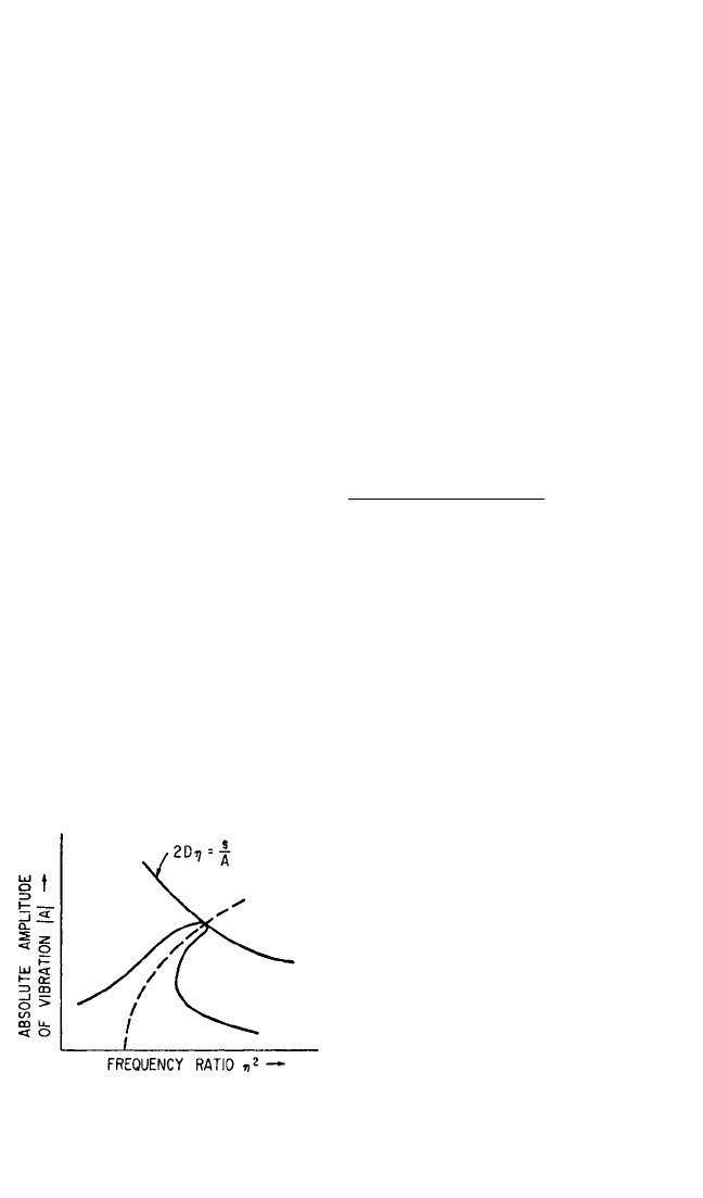
The maximum amplitude of vibration is of interest. The amplitude at the point at

which a response curve crosses the free vibration curve is termed the resonance

amplitude, and is determined in the nonlinear case by solving Eqs. (4.49) and (4.52)

simultaneously. This leads to

2Dη= θ= (4.54)

The first of these two equations defines

a hyperbola in the response diagram,

describing the locus of crossing points,

as shown in Fig. 4.25; hence, the intersec-

tion of this curve with the free vibration

curve gives the resonance amplitude.

The phase angle at resonance has the

value π/2, as in the linear case.This result

is of great help in computing response

curves since the effect of damping

(except for very large values) is negligi-

ble except in the neighborhood of reso-

nance.Therefore, one may compute only

the undamped curves (which is not diffi-

cult) and the hyperbola (which does not

contain the nonlinearity); then, the effect of damping may be sketched in from

knowledge of the crossing point.



∂F(A)



∂A



∂F(A)



∂A



2a





4.32 CHAPTER FOUR

FIGURE 4.25 Determination of the resonant

amplitude in accordance with Eq. (4.54).

8434_Harris_04_b.qxd 09/20/2001 11:30 AM Page 4.32

SYSTEM WITH GENERAL DAMPING AND

GENERAL RESTORING FORCES

The preceding analysis may be extended to include the more general differential

equation

E  ¨x + 2Dκg(˙x) +κ

f(x) − p cos ωt = 0

By procedures similar to those employed above:

[F(A) −η

]

+ 4D

(A) =



(4.55)

tan θ= (4.56)

where S(A) =



2π

g(ωA sin σ) sin σ dσ

In the case of linear velocity damping, S(A) =η, and Eqs. (4.55) and (4.56) reduce

to Eqs. (4.47) and (4.48). The results for various types of damping forces are:

Coulomb damping: g(˙x) =±υ

S(A) =

Linear velocity damping: g(˙x) =υ

˙xS(A) =υ

Velocity squared damping: g(˙x) =υ

˙x|˙x| S(A) =υ

2η

(Aω)

nth-power velocity damping: g(˙x) =υ

˙x|˙x|

n − 1

S(A) =υ

nη

(Aω)

n − 1

ϕ(n)

where ϕ(n) is defined in Eq. (4.41) and values are given in Table 4.1.

The locus of resonance amplitudes or crossing points is now given by

2DS(A) =θ=

GRAPHICAL METHODS OF INTEGRATION

Graphical methods (or their numerical equivalents) may be employed in the analy-

sis of nonlinear vibration and often prove to be of great value both for general stud-

ies of the behavior of a particular system and for actual integration of the equation

of motion.

A single degree-of-freedom system requires two parameters to describe com-

pletely the state of the motion. When these two parameters are used as coordinate

axes, the graphical representation of the motion is called a phase-plane representa-

tion. In dealing with ordinary dynamical problems, these parameters frequently are

taken as the displacement and velocity. First consider an undamped linear system

having the equation of motion

¨x +ω

x = 0 (4.57)

and the solution



3π



κA



πκA

2DS(A)



F(A) −η



NONLINEAR VIBRATION 4.33

8434_Harris_04_b.qxd 09/20/2001 11:30 AM Page 4.33

x = A cos ω

t + B sin ω

y ==−A sin ω

t + B cos ω

(4.58)

Eliminating time as a variable between Eqs. (4.58):

+ y

= c

Thus, the phase-plane representation is a family of concentric circles with centers at

the origin. Such curves are called trajectories. The necessary and sufficient conditions

in the phase-plane for periodic motions are (1) closed trajectories and (2) paths

described in finite time.

Now, suppose that the solution of Eq. (4.57) is not known. By introducing y = ˙x/ω

=ω

y =−ω

Therefore

=− (4.59)

Thus, the path in the phase-plane is described by a simple first-order differential

equation. This process of eliminating the time always can be done in principle, but

frequently the problem is too difficult. Since the time is to be eliminated, only

autonomous systems can be treated by phase-plane methods. When an equation of

the type of Eq. (4.59) can be found, a direct solution of the problem follows since

slopes of the trajectories can be sketched in the phase-plane and the trajectories

determined by connecting the tangents; this is known as the method of isoclines. It

sometimes happens that dx = 0, dy = 0 simultaneously so that there is no knowledge

of the direction of the motion; such points in the phase-plane are called singular

points. In the present example, the origin constitutes a singular point.

Consider now a damped linear system having the equation of motion

¨x + 2ζω

˙x +ω

x = 0

and the solution

x = Ce

−δt

cos Φ

(4.60)

y ==Ce

−δt

cos (Φ+σ)

where δ=ζω

=−ω

cos σ



σ>



Φ=υt +θ

υ=ω

1



−



=ω

sin σ

Equations (4.60) indicate that the trajectories in the phase-plane are some form of spi-

ral (one of the simplest known of which is the logarithmic spiral). By referring to the

oblique coordinate system shown in Fig. 4.26, and recalling that sin σ is a constant and

= x

+ y

− 2xy cos σ

Eqs. (4.60) reduce to



˙x



˙x



4.34 CHAPTER FOUR

8434_Harris_04_b.qxd 09/20/2001 11:30 AM Page 4.34