Harris C.M., Piersol A.G. Harris Shock and vibration handbook

Подождите немного. Документ загружается.

The analogy represented by Eqs. (8.1b), (8.1d), and (8.1e) may be extended fur-

ther since it is generally possible to differentiate Eq. (8.1b) any number of times n:



(t) (8.1f )

This is of the same general form as the preceding equations if it is considered to be

a second-order equation in (d

x/dt

) as the response variable, with (d

u/dt

) (t), a

known function of time, as the excitation.

ALTERNATE FORMS OF THE EXCITATION AND OF THE RESPONSE

The foregoing equations are alike, mathematically, and a solution in terms of one of

them may be applied to any of the others by making simple substitutions.Therefore,

the equations may be expressed in the single general form:

¨ν+ν=ξ(t) (8.2)

where ν and ξ are the response and the excitation, respectively, at time t.

A general notation (ν and ξ) is desirable in the presentation of response func-

tions and response spectra for general use. However, in the discussion of examples

of solution, it sometimes is preferable to use more specific notations. Both types of

notation are used in this chapter. For ready reference, the alternate forms of the

excitation and the response are given in Table 8.1 where

= k/m.

METHODS OF SOLUTION OF THE DIFFERENTIAL EQUATION

A brief review of four methods of solution is given in the following sections.

Classical Solution. The complete solution of the linear differential equation of

motion consists of the sum of the particular integral x

and the complementary func-

tion x

, that is, x = x

+ x

. Since the differential equation is of second order, two con-



TRANSIENT RESPONSE TO STEP AND PULSE FUNCTIONS 8.3

TABLE 8.1 Alternate Forms of Excitation and Response in Eq. (8.2)

Excitation ξ(t) Response ν

Force Absolute displacement x

Ground displacement u(t) Absolute displacement x

Ground acceleration Relative displacement δ

Ground acceleration ü(t) Absolute acceleration ¨x

Ground velocity ˙u(t) Absolute velocity ˙x

nth derivative of (t) nth derivative of

ground displacement absolute displacement



−ü(t)



F(t)



8434_Harris_08_b.qxd 09/20/2001 11:19 AM Page 8.3

stants of integration are involved. They appear in the complementary function and

are evaluated from a knowledge of the initial conditions.

Example 8.1: Versed-sine Force Pulse. In this case the differential equation of

motion, applicable for the duration of the pulse, is

+ x =



1 − cos



[0 ≤ t ≤τ] (8.3a)

where, in terms of the general notation, the excitation function ξ(t) is

ξ(t)  =



1 − cos



and the response ν is displacement x. The maximum value of the pulse excitation

force is F

The particular integral (particular solution) for Eq. (8.3a) is of the form

= M + N cos (8.3b)

By substitution of the particular solution into the differential equation, the required

values of the coefficients M and N are found.

The complementary function is

= A cos ω

t + B sin ω

t (8.3c)

where A and B are the constants of integration. Combining x

and the explicit form

of x

gives the complete solution:

x = x

+ x



1 −+cos



+ A cos ω

t + B sin ω

t (8.3d)

If it is assumed that the system is initially at rest, x = 0 and ˙x = 0 at t = 0, and the

constants of integration are

A =− and B = 0 (8.3e)

The complete solution takes the following form:

ν  x =



1 −+cos − cos ω



(8.3f )

If other starting conditions had been assumed, A and B would have been differ-

ent from the values given by Eqs. (8.3e). It may be shown that if the starting condi-

tions are general, namely, x = x

and ˙x = x

at t = 0, it is necessary to superimpose on

the complete solution already found, Eq. (8.3f), only the following additional terms:

cos ω

t + sin ω

t (8.3g)

For values of time equal to or greater than τ, the differential equation is

m¨x + kx = 0[τ≤t] (8.4a)

and the complete solution is given by the complementary function alone. However,

the constants of integration must be redetermined from the known conditions of the

system at time t =τ. The solution is

˙x



2πt



/2k



1 −τ

/2k



1 −τ

2πt



/2k



1 −τ

2πt



2πt



F(t)



2πt



m¨x



8.4 CHAPTER EIGHT

8434_Harris_08_b.qxd 09/20/2001 11:19 AM Page 8.4

ν  x = sin ω



t −



[τ≤t] (8.4b)

The additional terms given by expressions (8.3g) may be superimposed on this solu-

tion if the conditions at time t = 0 are general.

Duhamel’s Integral. The use of Du-

hamel’s integral (convolution integral or

superposition integral) is a well-known

approach to the solution of transient

vibration problems in linear systems. Its

development

is based on the superposi-

tion of the responses of the system to a

sequence of impulses.

A general excitation function is

shown in Fig. 8.2, where F(t) is a known

force function of time, the variable of

integration is t

between the limits of

integration 0 and t, and the elemental

impulse is F(t

) dt

. It may be shown that the complete solution of the differential

equation is

x =



− 

F(t

) sin ω



cos ω

t +



+ 

F(t

) cos ω



sin ω

(8.5)

where x

and ˙x

are the initial conditions of the system at zero time.

Example 8.2: Half-cycle Sine, Ground Displacement Pulse. Consider the fol-

lowing excitation:

ξ(t)  u(t) =



sin [0 ≤ t ≤τ]

0[τ≤t]

The maximum value of the excitation displacement is u

. Assume that the system is

initially at rest, so that x

= ˙x

= 0. Expressing the excitation function in terms of the

variable of integration t

, Eq. (8.5) may be rewritten for this particular case in the fol-

lowing form:

x =



− cos ω

t 

sin sin ω

+ sin ω

t 

sin cos ω



(8.6a)

Equation (8.6a) may be reduced, by evaluation of the integrals, to

ν  x =



sin − sin ω



[0 ≤ t ≤τ] (8.6b)

where T = 2π/ω

is the natural period of the responding system.

For the second era of time, where τ≤t, it is convenient to choose a new time vari-

able t′=t −τ. Noting that u(t) = 0 for τ≤t, and that for continuity in the system

response the initial conditions for the second era must equal the closing conditions

for the first era, it is found from Eq. (8.5) that the response for the second era is



2τ

πt





1 − T

/4τ

πt



πt



mω

πt



mω

¨x



mω



sin (πτ/T)



1 −τ



TRANSIENT RESPONSE TO STEP AND PULSE FUNCTIONS 8.5

FIGURE 8.2 General excitation and the ele-

mental impulse.

8434_Harris_08_b.qxd 09/20/2001 11:19 AM Page 8.5

x = x

cos ω

t′+ sin ω

t′ (8.7a)

where x

and ˙x

are the displacement and velocity of the system at time t =τand

hence at t′=0. Equation (8.7a) may be rewritten in the following form:

ν  x = u

sin ω



t −



[τ≤t] (8.7b)

Phase-Plane Graphical Method. Several numerical and graphical methods,

18, 23

all

related in general but differing considerably in the details of procedure, are available

for the solution of linear transient vibration problems. Of these methods, the phase-

plane graphical method is one of the

most useful. The procedure is basically

very simple, it gives a clear physical pic-

ture of the response of the system, and it

may be applied readily to some classes of

nonlinear systems.

3, 5, 6, 8, 13, 15, 21, 22

In Fig. 8.3 a general excitation in

terms of ground displacement is repre-

sented, approximately, by a sequence of

finite steps. The ith step has the total

height u

, where u

is constant for the

duration of the step. The differential

equation of motion and its complete

solution, applying for the duration of the

step, are

+ x = u

i − 1

≤ t ≤ t

] (8.8a)

x − u

= (x

i − 1

− u

) cos ω

(t − t

i − 1

) + sin ω

(t − t

i − 1

) (8.8b)

where x

i − 1

and ˙x

i − 1

are the displacement and velocity of the system at time t

i − 1

;

consequently, they are the initial conditions for the ith step. The system velocity

(divided by ω

) during the ith step is

=−(x

i − 1

− u

) sin ω

(t − t

i − 1

) + cos ω

(t − t

i − 1

) (8.8c)

Squaring Eqs. (8.8b) and (8.8c) and adding them,



+ (x − u

)



+ (x

i − 1

− u

)

(8.8d)

This is the equation of a circle in a rectangular system of coordinates ˙x/ω

, x. The

center is at 0, u

; and the radius is

 

+ (x

i − 1

− u

)



1/2

(8.8e)

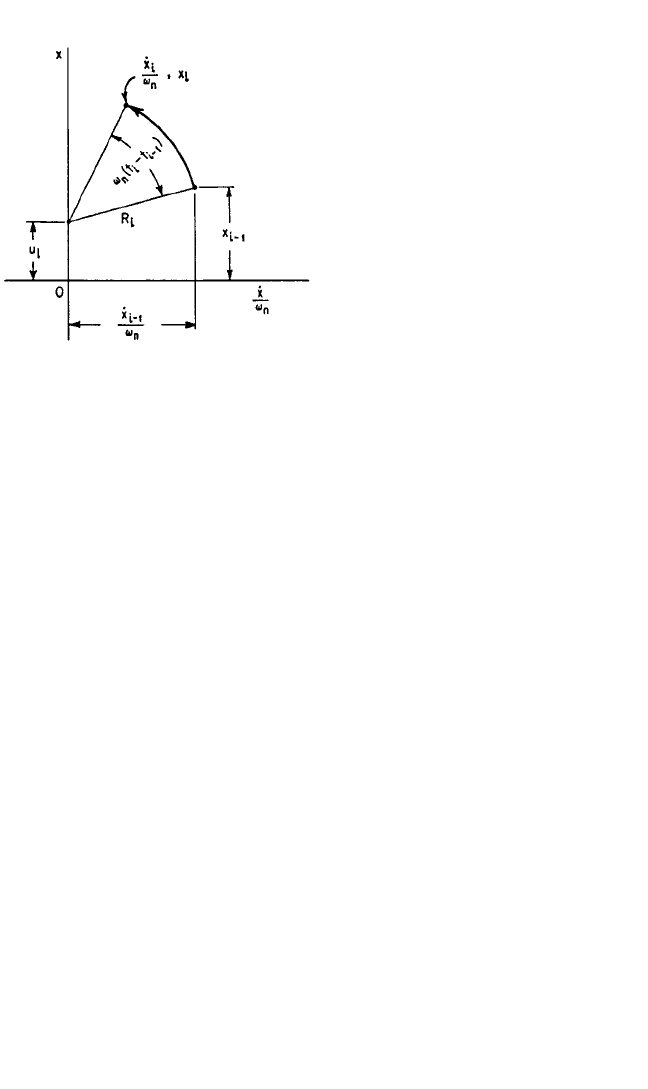
The solution for Eq. (8.8a) for the ith step may be shown, as in Fig. 8.4, to be the

arc of the circle of radius R

and center 0, u

, subtended by the angle ω

− t

i − 1

) and

starting at the point ˙x

i − 1

/ω

, x

i − 1

.Time is positive in the counterclockwise direction.

˙x

i − 1



˙x

i − 1



˙x



˙x

i − 1



˙x



˙x

i − 1



m¨x



(T/τ) cos (πτ/T)



/4τ

) − 1

˙x



8.6 CHAPTER EIGHT

FIGURE 8.3 General excitation approxi-

mated by a sequence of finite rectangular steps.

8434_Harris_08_b.qxd 09/20/2001 11:19 AM Page 8.6

Example 8.3: Application to a

General Pulse Excitation. Figure 8.5

shows an application of the method for

the general excitation u(t) represented

by seven steps in the time-displacement

plane. Upon choice of the step heights u

and durations (t

− t

i − 1

), the arc-center

locations can be projected onto the X

axis in the phase-plane and the arc

angles ω

− t

i − 1

) can be computed.The

graphical construction of the sequence

of circular arcs, the phase trajectory, is

then carried out, using the system condi-

tions at zero time (in this example, 0,0)

as the starting point.

Projection of the system displace-

ments from the phase-plane into the

time-displacement plane at once deter-

mines the time-displacement response

curve. The time-velocity response can also be determined by projection as shown.

The velocities and displacements at particular instants of time can be found directly

from the phase trajectory coordinates without the necessity for drawing the time-

response curves. Furthermore, the times of occurrence and the magnitudes of all the

maxima also can be obtained directly from the phase trajectory.

Good accuracy is obtainable by using reasonable care in the graphical construc-

tion and in the choice of the steps representing the excitation. Usually, the time inter-

vals should not be longer than about one-fourth the natural period of the system.

The Laplace Transformation. The Laplace transformation provides a powerful

tool for the solution of linear differential equations. The following discussion of the

technique of its application is limited to the differential equation of the type apply-

ing to the undamped linear oscillator. Application to the linear oscillator with vis-

cous damping is illustrated in a later part of this chapter.

Definitions. The Laplace transform F(s) of a known function f(t), where t > 0, is

defined by

F(s) =



∞

−st

f(t)dt (8.9a)

where s is a complex variable. The transformation is abbreviated as

F(s) = L[f(t)] (8.9b)

The limitations on the function f(t) are not discussed here. For the conditions

for existence of L[f(t)], for complete accounts of the technique of application, and

for extensive tables of function-transform pairs, the references should be con-

sulted.

16, 17

General Steps in Solution of the Differential Equation. In the solution of a

differential equation by Laplace transformation, the first step is to transform the dif-

ferential equation, in the variable t, into an algebraic equation in the complex vari-

able s. Then, the algebraic equation is solved, and the solution of the differential

equation is determined by an inverse transformation of the solution of the algebraic

equation. The process of inverse Laplace transformation is symbolized by

TRANSIENT RESPONSE TO STEP AND PULSE FUNCTIONS 8.7

FIGURE 8.4 Graphical representation in the

phase-plane of the solution for the ith step.

8434_Harris_08_b.qxd 09/20/2001 11:19 AM Page 8.7

−1

[F(s)] = f(t) (8.10)

Tables of Function-Transform Pairs. The processes symbolized by Eqs. (8.9b)

and (8.10) are facilitated by the use of tables of function-transform pairs.Table 8.2 is

a brief example. Transforms for general operations, such as differentiation, are

included as well as transforms of explicit functions.

In general, the transforms of the explicit functions can be obtained by carrying

out the integration indicated by the definition of the Laplace transformation. For

example:

For f(t) = 1:

F(s) =



∞

−st

dt =− e

−st



∞



8.8 CHAPTER EIGHT

FIGURE 8.5 Example of phase-plane graphical solution.

8434_Harris_08_b.qxd 09/20/2001 11:19 AM Page 8.8

TABLE 8.2 Pairs of Functions f(t) and Laplace Transforms F(s)

8.9

8434_Harris_08_b.qxd 09/20/2001 11:19 AM Page 8.9

Transformation of the Differential Equation. The differential equation for the

undamped linear oscillator is given in general form by

¨ν+ν=ξ(t) (8.11)

Applying the operational transforms (items 1 and 3, Table 8.2), Eq. (8.11) is trans-

formed to

(s) − sf(0) − f′(0) + F

(s) = F

(s) (8.12a)

where F

(s) = the transform of the unknown response ν(t),

sometimes called the response transform

(s) − sf(0) − f′(0) = the transform of the second derivative of ν(t)

f(0) and f′(0) = the known initial values of ν and ˙ν, i.e., ν

and ˙ν

(s) = the transform of the known excitation function ξ(t),

written F

(s) = L[ξ(t)], sometimes called the driving

transform

It should be noted that the initial conditions of the system are explicit in Eq. (8.12a).

The Subsidiary Equation. Solving Eq. (8.12a) for F

(s),

(s) = (8.12b)

This is known as the subsidiary equation of the differential equation. The first two

terms of the transform derive from the initial conditions of the system, and the third

term derives from the excitation.

Inverse Transformation. In order to determine the response function ν(t),

which is the solution of the differential equation, an inverse transformation is per-

formed on the subsidiary equation. The entire operation, applied explicitly to the

solution of Eq. (8.11), may be abbreviated as follows:

ν(t) = L

−1

(s)] = L

−1



(8.13)

Example 8.4: Rectangular Step Excitation. In this case ξ(t) =ξ

for 0 ≤ t (Fig.

8.6A). The Laplace transform F

(s) of the excitation is, from item 7 of Table 8.2,

L[ξ

] =ξ

L[1] =ξ

Assume that the starting conditions are general, that is, ν=ν

and ˙ν=˙ν

at t = 0. Sub-

stituting the transform and the starting conditions into Eq. (8.13), the following is

obtained:

ν(t) = L

−1



(8.14a)

The foregoing may be rewritten as three separate inverse transforms:

ν(t) =ν

−1



+ ˙ν

−1



+ξ

−1



(8.14b)

The inverse transforms in Eq. (8.14b) are evaluated by use of items 19, 12 and 13,

respectively, in Table 8.2. Thus, the time-response function is given explicitly by



s(s

)



sν

+ ˙ν

(1/s)





sν

+ ˙ν

+ω

L[ξ(t)]



sf(0) + f′(0) +ω

(s)



+ω



8.10 CHAPTER EIGHT

8434_Harris_08_b.qxd 09/20/2001 11:19 AM Page 8.10

ν(t) =ν

cos ω

t + sin ω

t +ξ

(1 − cos ω

t) (8.14c)

The first two terms are the same as the starting condition response terms given by

expressions (8.20a). The third term agrees with the response function shown by Eq.

(8.22), derived for the case of a start from rest.

Example 8.5: Rectangular Pulse Excitation. The excitation function, Fig.

8.6B, is given by

ξ(t) =



for 0 ≤ t ≤τ

0 for τ≤t

For simplicity, assume a start from rest, i.e., ν

= 0 and ˙ν

= 0 when t = 0.

During the first time interval, 0 ≤ t ≤τ, the response function is of the same form as

Eq. (8.14c) except that, with the assumed start from rest, the first two terms are zero.

During the second interval, τ≤t, the transform of the excitation is obtained by

applying the delayed-function transform (item 6, Table 8.2) and the transform for

the rectangular step function (item 7) with the following result:

˙ν



TRANSIENT RESPONSE TO STEP AND PULSE FUNCTIONS 8.11

FIGURE 8.6 Excitation functions in examples of use of the

Laplace transform: (A) rectangular step, (B) rectangular pulse, (C)

step with constant-slope front, (D) sine pulse, and (E) step with

exponential asymptotic rise.

8434_Harris_08_b.qxd 09/20/2001 11:20 AM Page 8.11

(s) = L[ξ(t)] =ξ



−



This is the transform of an excitation consisting of a rectangular step of height −ξ

starting at time t =τ, superimposed on the rectangular step of height +ξ

starting at

time t = 0.

Substituting for L[ξ(t)] in Eq. (8.13),

ν(t) =ξ



−1



− L

−1



(8.15a)

The first inverse transform in Eq. (8.15a) is the same as the third one in Eq. (8.14b)

and is evaluated by use of item 13 in Table 8.2. However, the second inverse trans-

form requires the use of items 6 and 13. The function-transform pair given by item 6

indicates that when t < b the inverse transform in question is zero, and when t > b the

inverse transform is evaluated by replacing t by t − b (in this particular case, by t −τ).

The result is as follows:

ν(t) =ξ



(1 − cos ω

t) − [1 − cos ω

(t −τ)]



= 2ξ

sin sin ω



t −



[τ≤t] (8.15b)

Theorem on the Transform of Functions Shifted in the Original (t) Plane. In

Example 8.5, use is made of the theorem on the transform of functions shifted in

the original plane. The theorem (item 6 in Table 8.2) is known variously as the

second shifting theorem, the theorem on the transform of delayed functions, and

the time-displacement theorem. In determining the transform of the excitation, the

theorem provides for shifting, i.e., displacing the excitation or a component of the

excitation in the positive direction along the time axis.This suggests the term delayed

function. Examples of the shifting of component parts of the excitation appear in

Fig. 8.6B, 8.6C, and 8.6D. Use of the theorem also is necessary in determining, by

means of inverse transformation, the response following the delay in the excitation.

Further illustration of the use of the theorem is shown by the next two examples.

Example 8.6: Step Function with Constant-slope Front. The excitation func-

tion (Fig. 8.6C) is expressed as follows:

ξ(t) =



[0 ≤ t ≤τ]

[τ≤t]

Assume that ν

= 0 and ˙ν

= 0.

The driving transforms for the first and second time intervals are

L[ξ(t)] =



[0 ≤ t ≤τ]



−



[τ≤t]

The transform for the second interval is the transform of a negative constant slope

excitation, −ξ

(t −τ)/τ, starting at t =τ, superimposed on the transform for the posi-

tive constant slope excitation, +ξ

t/τ, starting at t = 0.

−sτ



πτ



−sτ



s(s

)



s(s

)

−sτ



8.12 CHAPTER EIGHT

8434_Harris_08_b.qxd 09/20/2001 11:20 AM Page 8.12