Hirsch M., Smale S., Devaney R., Differential Equations, Dynamical Systems, and an Introduction to Chaos
Подождите немного. Документ загружается.


286 Chapter 13 Applications in Mechanics
We visualize phase space as the collection of all tangent vectors at each point
X ∈
C. For a given X ∈ R
2
−{0}, let T
X
={(X , V ) |V ∈ R
2
}. T
X
is the
tangent plane to the configuration space at X . Then
P =
X∈C
T
X
is the tangent space to the configuration space, which we may naturally identify
with a subset of
R
4
.
The dimension of phase space is four. However, we can cut this dimension
in half by making use of the two known first integrals, total energy and angu-
lar momentum. Recall that energy is constant along solutions and is given by
E(X , V ) = K (V ) + U (X ) =
1
2
|V |
2
−
1
|X|
.
Let
h
denote the subset of P consisting of all points (X, V ) with E(X, V ) = h.
The set
h
is called an energy surface with total energy h.Ifh ≥ 0, then
h
meets each T
X
in a circle of tangent vectors satisfying
|V |
2
= 2
h +
1
|X|
.
The radius of these circles in the tangent planes at X tends to ∞as X → 0 and
decreases to 2h as |X | tends to ∞.
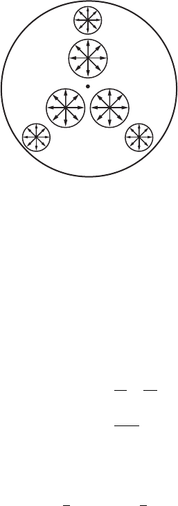
When h<0, the structure of the energy surface
h
is different. If |X | >
−1/h, then there are no vectors in T
X
∩
h
. When |X |=−1/h, only the zero
vector in T
X
lies in
h
. The circle r =−1/h in configuration space is therefore
known as the zero velocity curve.IfX lies inside the zero velocity curve, then
T
X
meets the energy surface in a circle of tangent vectors as before. Figure 13.1
gives a caricature of
h
for the case where h<0.
We now introduce polar coordinates in configuration space and new
variables (v
r
, v
θ
) in the tangent planes via
V = v
r
cos θ
sin θ
+ v
θ
−sin θ
cos θ
.
We have
V = X
= r
cos θ
sin θ
+ rθ
−sin θ
cos θ
so that r
= v
r
and θ
= v
θ
/r. Differentiating once more, we find
−1
r
2
cosθ
sinθ
=−
X
|X|
3
=V
=
v
r
−
v
2
θ
r
cosθ
sinθ
+
v
r
v
θ
r
+v
θ
−sinθ
cosθ
.
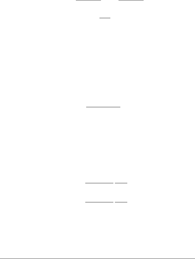
13.4 The Newtonian Central Force System 287
zero velocity
curve
Figure 13.1 Over each nonzero point
inside the zero velocity curve, T
X
meets the energy surface
h
in a circle
of tangent vectors.
Therefore in the new coordinates (r,θ ,v
r
,v
θ
), the system becomes
r
=v
r
θ
=v
θ
/r
v
r
=−
1
r
2
+
v
2
θ
r
v
θ
=−
v
r
v
θ
r
.
In these coordinates, total energy is given by
1
2
v
2
r
+v
2
θ
−
1
r
=h
and angular momentum is given by =rv
θ
. Let
h,
consist of all points in
phase space with total energy h and angular momentum . For simplicity, we
will restrict attention to the case where h<0.
If =0, we must have v
θ
=0. So if X lies inside the zero velocity curve, the
tangent space at X meets
h,0
in precisely two vectors of the form
±v
r
cosθ
sinθ
,
both of which lie on the line connecting 0 and X, one pointing toward 0, the
other pointing away. On the zero velocity curve, only the zero vector lies in
h,0
. Hence we see immediately that each solution in
h,0
lies on a straight line

288 Chapter 13 Applications in Mechanics
through the origin. The solution leaves the origin and travels along a straight
line until reaching the zero velocity curve, after which time it recedes back to
the origin. In fact, since the vectors in
h,0
have magnitude tending to ∞ as
X →0, these solutions reach the singularity in finite time in both directions.
Solutions of this type are called collision-ejection orbits.
When =0, a different picture emerges. Given X inside the zero velocity
curve, we have v
θ
=/r, so that, from the total energy formula,
r
2
v
2
r
=2hr
2
+2r −
2
. (A)
The quadratic polynomial in r on the right in Eq. (A) must therefore be
nonnegative, so this puts restrictions on which r-values can occur for X ∈
h,
.
The graph of this quadratic polynomial is concave down since h<0. It has no
real roots if
2
> −1/2h. Therefore the space
h,
is empty in this case. If
2
=−1/2h, we have a single root that occurs at r =−1/2h. Hence this is the
only allowable r-value in
h,
in this case. In the tangent plane at (r, θ), we
have v
r
=0, v
θ
=−2h, so this represents a circular closed orbit (traversed
clockwise if < 0, counterclockwise if > 0).
If
2
< −1/2h, then this polynomial has a pair of distinct roots at α,β with
α < −1/2h<β. Note that α > 0. Let A
α,β
be the annular region α ≤r ≤β in
configuration space. We therefore have that motion in configuration space is
confined to A
α,β
.
Proposition. Suppose h <0 and
2
< −1/2h. Then
h,
⊂P is a two-
dimensional torus.
Proof: We compute the set of tangent vectors lying in T
X
∩
h,
for each
X ∈A
α,β
.IfX lies on the boundary of the annulus, the quadratic term on the
right of Eq. (A) vanishes, and so v
r
=0 while v
θ
=/r. Hence there is a unique
tangent vector in T
X
∩
h,
when X lies on the boundary of the annulus. When
X is in the interior of A
α,β
, we have
v
±
r
=±
1
r
2hr
2
+2r −
2
, v
θ
=/r
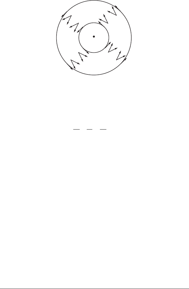
so that we have a pair of vectors in T
X
∩
h,
in this case. Note that these
vectors all point either clockwise or counterclockwise in A
α,β
, since v
θ
has the
same sign for all X . See Figure 13.2. Thus we can think of
h,
as being given
by a pair of graphs over A
α,β
: a positive graph given by v
+
r
and a negative
graph given by v
−
r
which are joined together along the boundary circles r =α
and r =β. (Of course, the “real” picture is a subset of
R
4
.) This yields the
torus.
It is tempting to think that the two curves in the torus given by r =α and
r =β are closed orbits for the system, but this is not the case. This follows
13.5 Kepler’s First Law 289
A
a,b
Figure 13.2 A selection of
vectors in
h
,
.
since, when r =α, we have
v
r
=−
1
α
2
+
v
2
θ
α
=
1
α
3
(−α+
2
).
However, since the right-hand side of Eq. (A) vanishes at α, we have
2hα
2
+2α −
2
=0,
so that
−α+
2
=(2hα +1)α.
Since α < −1/2h, it follows that r
=v
r
> 0 when r =α, so the r coordinate of
solutions in
h,
reaches a minimum when the curve meets r =α. Similarly,
along r =β, the r coordinate reaches a maximum.
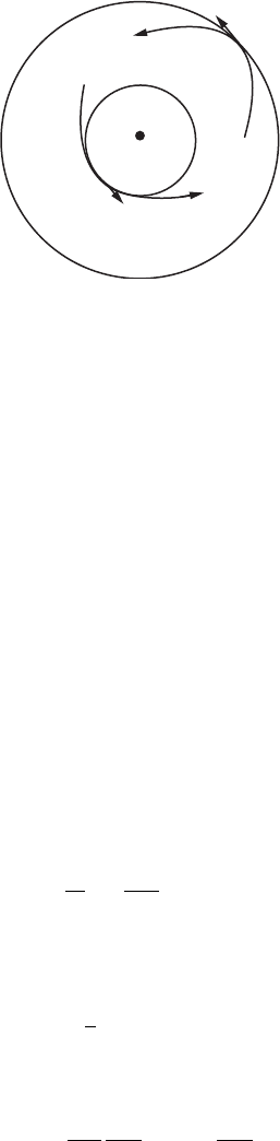
Hence solutions in A
α,β
must behave as shown in Figure 13.3. As a remark,
one can easily show that these curves are preserved by rotations about the
origin, so all of these solutions behave symmetrically.
More, however, can be said. Each of these solutions actually lies on a closed
orbit that traces out an ellipse in configuration space. To see this, we need to
turn to analysis.
13.5 Kepler’s First Law
For most nonlinear mechanical systems, the geometric analysis of the previous
section is just about all we can hope for. In the Newtonian central force system,
290 Chapter 13 Applications in Mechanics
A
a,
b
Figure 13.3 Solutions in
h
,
that meet r = α or r = β.
however, we get lucky: As has been known for centuries, we can write down
explicit solutions for this system.
Consider a particular solution curve of the differential equation. We have
two constants of the motion for this system, namely, the angular momentum
and total energy E. The case =0 yields collision-ejection solutions as we
saw above. Hence we assume =0. We will show that in polar coordinates
in configuration space, a solution with nonzero angular momentum lies on a
curve given by r(1+ cosθ) =κ where and κ are constants. This equation
defines a conic section, as can be seen by rewriting this equation in Cartesian
coordinates. This fact is known as Kepler’s first law.
To prove this, recall that r
2
θ
is constant and nonzero. Hence the sign of
θ
remains constant along each solution curve. Thus θ is always increasing or
always decreasing in time. Therefore we may also regard r as a function of θ
along the curve.
Let W (t ) =1/r(t ); then W is also a function of θ. Note that W =−U . The
following proposition gives a convenient formula for kinetic energy.
Proposition. The kinetic energy is given by
K =
2
2
dW
dθ
2
+W
2
.
Proof: In polar coordinates, we have
K =
1
2
(r
)
2
+(rθ
)
2
.
Since r =1/W , we also have
r
=
−1
W
2
dW
dθ
θ
=−
dW
dθ
.
13.5 Kepler’s First Law 291
Finally,
rθ
=
r
=W .
Substitution into the formula for K then completes the proof.
Now we find a differential equation relating W and θ along the solution
curve. Observe that K =E −U =E +W . From the proposition we get
dW
dθ
2
+W
2
=
2
2
(E +W ). (B)
Differentiating both sides with respect to θ, dividing by 2 dW /dθ, and using
dE/dθ =0 (conservation of energy), we obtain
d
2
W
dθ
2
+W =
1
2
where 1/
2
is a constant.
Note that this equation is just the equation for a harmonic oscillator with
constant forcing 1/
2
. From elementary calculus, solutions of this second-
order equation can be written in the form
W (θ) =
1
2
+A cos θ +B sin θ
or, equivalently,
W (θ) =
1
2
+C cos
(
θ +θ
0
)
where the constants C and θ
0
are related to A and B.
If we substitute this expression into Eq. (B) and solve for C (at, say, θ +θ
0
=
π/2), we find
C =±
1
2
1+2
2
E.
Inserting this into the solution above, we find
W (θ) =
1
2
1±
1+2E
2
cos(θ +θ
0
)
.
There is no need to consider both signs in front of the radical since
cos(θ +θ
0
+π ) =−cos(θ +θ
0
).

292 Chapter 13 Applications in Mechanics
Moreover, by changing the variable θ to θ −θ
0
we can put any particular
solution into the form
1
2
1+
1+2E
2
cosθ
.
This looks pretty complicated. However, recall from analytic geometry (or
from Exercise 2 at the end of this chapter) that the equation of a conic in polar
coordinates is
1
r
=
1
κ
(1+ cos θ).
Here κ is the latus rectum and ≥0istheeccentricity of the conic. The origin
is a focus and the three cases > 1, =1, < 1 correspond, respectively, to
a hyperbola, parabola, and ellipse. The case =0 is a circle. In our case we
have
=
1+2E
2
,
so the three different cases occur when E>0, E =0, or E<0. We have proved:
Theorem. (Kepler’s First Law) The path of a particle moving under the
influence of Newton’s law of gravitation is a conic of eccentricity
1+2E
2
.
This path lies along a hyperbola, parabola, or ellipse according to whether E > 0,
E =0,orE<0.
13.6 The Two-Body Problem
We now turn our attention briefly to what at first appears to be a more difficult
problem, the two-body problem. In this system we assume that we have two
masses that move in space according to their mutual gravitational attraction.
Let X
1
,X
2
denote the positions of particles of mass m
1
,m
2
in R
3
.SoX
1
=
(x
1
1
,x
1
2
,x
1
3
) and X
2
=(x
2
1
,x
2
2
,x
2
3
). From Newton’s law of gravitation, we find
the equations of motion
m
1
X
1
=gm
1
m
2
X
2
−X
1
|X
2
−X
1
|
3
m
2
X
2
=gm
1
m
2
X
1
−X
2
|X
1
−X
2
|
3
.
13.7 Blowing Up the Singularity 293
Let’s examine these equations from the perspective of a viewer living on the
first mass. Let X =X
2
−X
1
. We then have
X
=X
2
−X
1
=gm
1
X
1
−X
2
|X
1
−X
2
|
3
−gm
2
X
2
−X
1
|X
1
−X
2
|
3
=−g (m
1
+m
2
)
X
|X|
3
.
But this is just the Newtonian central force problem, with a different choice of
constants.
So, to solve the two-body problem, we first determine the solution of X(t )
of this central force problem. This then determines the right-hand side of the
differential equations for both X
1
and X
2
as functions of t, and so we can
simply integrate twice to find X
1
(t) and X
2
(t).
Another way to reduce the two-body problem to the Newtonian central
force is as follows. The center of mass of the two-body system is the vector
X
c
=
m
1
X
1
+m
2
X
2
m
1
+m
2
.
A computation shows that X
c
=0. Therefore we must have X
c
=At +B where
A and B are fixed vectors in
R
3
. This says that the center of mass of the system
moves along a straight line with constant velocity.
We now change coordinates so that the origin of the system is located at X
c
.
That is, we set Y
j
=X
j
−X
c
for j =1,2. Therefore m
1
Y
1
(t)+m
2
Y
2
(t) =0 for all
t. Rewriting the differential equations in terms of the Y
j
,wefind
Y
1
=−
gm
3
2
(m
1
+m
2
)
3
Y
1
|Y
1
|
3
Y
2
=−
gm
3
1
(m
1
+m
2
)
3
Y
2
|Y
2
|
3
,
which yields a pair of central force problems. However, since we know that
m
1
Y
1
(t)+m
2
Y
2
(t) =0, we need only solve one of them.
13.7 Blowing Up the Singularity
The singularity at the origin in the Newtonian central force problem is the first
time we have encountered such a situation. Usually our vector fields have been
294 Chapter 13 Applications in Mechanics
well defined on all of R
n
. In mechanics, such singularities can sometimes be
removed by a combination of judicious changes of variables and time scalings.
In the Newtonian central force system, this may be achieved using a change of
variables introduced by McGehee [32].
We first introduce scaled variables
u
r
=r
1/2
v
r
u
θ
=r
1/2
v
θ
.
In these variables the system becomes
r
=r
−1/2
u
r
θ
=r
−3/2
u
θ
u
r
=r
−3/2
1
2
u
2
r
+u
2
θ
−1
u
θ
=r
−3/2
−
1
2
u
r
u
θ
.
We still have a singularity at the origin, but note that the last three equations
are all multiplied by r
−3/2
. We can remove these terms by simply multiplying
the vector field by r
3/2
. In doing so, solution curves of the system remain the
same but are parameterized differently.
More precisely, we introduce a new time variable τ via the rule
dt
dτ
=r
3/2
.
By the chain rule we have
dr
dτ
=
dr
dt
dt
dτ
and similarly for the other variables. In this new timescale the system
becomes
˙r =ru
r
˙
θ =u
θ
˙u
r
=
1
2
u
2
r
+u
2
θ
−1
˙u
θ
=−
1
2
u
r
u
θ

13.7 Blowing Up the Singularity 295
where the dot now indicates differentiation with respect to τ . Note that, when
r is small, dt /dτ is close to zero, so “time” τ moves much more slowly than
time t near the origin.
This system no longer has a singularity at the origin. We have “blown up”
the singularity and replaced it with a new set given by r =0 with θ,u
r
, and u
θ
being arbitrary. On this set the system is now perfectly well defined. Indeed,
the set r =0 is an invariant set for the flow since ˙r =0 when r =0. We have thus
introduced a fictitious flow on r =0. While solutions on r =0 mean nothing
in terms of the real system, by continuity of solutions, they can tell us a lot
about how solutions behave near the singularity.
We need not concern ourselves with all of r =0 since the total energy relation
in the new variables becomes
hr =
1
2
u
2
r
+u
2
θ
−1.
On the set r =0, only the subset defined by
u
2
r
+u
2
θ
=2, θ arbitrary
matters. The set is called the collision surface for the system; how solu-
tions behave on dictates how solutions move near the singularity since any
solution that approaches r =0 necessarily comes close to in our new coor-
dinates. Note that is a two-dimensional torus: It is formed by a circle in the
θ direction and a circle in the u
r
u
θ
–plane.
On the system reduces to
˙
θ =u
θ
˙u
r
=
1
2
u
2
θ
˙u
θ
=−
1
2
u
r
u
θ
where we have used the energy relation to simplify ˙u
r
. This system is easy
to analyze. We have ˙u
r
> 0 provided u
θ
=0. Hence the u
r
coordinate must
increase along any solution in with u
θ
=0.
On the other hand, when u
θ
=0, the system has equilibrium points. There
are two circles of equilibria, one given by u
θ
=0,u
r
=
√
2, and θ arbitrary, the
other by u
θ
=0,u
r
=−
√
2, and θ arbitrary. Let C
±
denote these two circles
with u
r
=±
√
2onC
±
. All other solutions must travel from C
−
to C
+
since
v
θ
increases along solutions.