Jacques I. Mathematics for Economics and Business
Подождите немного. Документ загружается.

Linear Equations
100
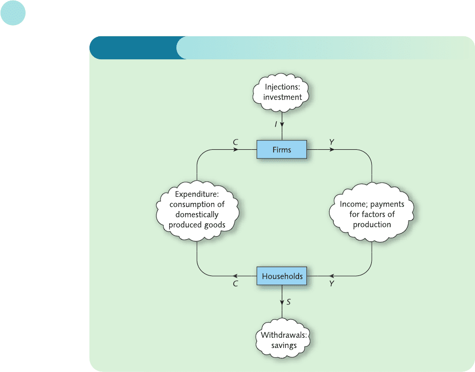
Let us examine this more closely and represent the diagrammatic information in symbols.
Consider first the box labelled ‘Households’. The flow of money entering this box is Y and the
flow leaving it is C + S. Hence we have the familiar relation
Y = C + S
For the box labelled ‘Firms’ the flow entering it is C + I and the flow leaving it is Y, so
Y = C + I
Suppose that the level of investment that firms plan to inject into the economy is known to be
some fixed value, I* . If the economy is in equilibrium, the flow of income and expenditure
balance so that
Y = C + I*
From the assumption that the consumption function is
C = aY + b
for given values of a and b these two equations represent a pair of simultaneous equations for
the two unknowns Y and C. In these circumstances C and Y can be regarded as endogenous
variables, since their precise values are determined within the model, whereas I* is fixed out-
side the model and is exogenous.
Figure 1.27
MFE_C01f.qxd 16/12/2005 10:58 Page 100

1.6 • National income determination
101
To make the model more realistic let us now include government expenditure, G, and
taxation, T, in the model. The injections box in Figure 1.27 now includes government expendi-
ture in addition to investment, so
Example
Find the equilibrium level of income and consumption if the consumption function is
C = 0.6Y + 10
and planned investment I = 12.
Solution
We know that
Y = C + I (from theory)
C = 0.6Y + 10 (given in problem)
I = 12 (given in problem)
If the value of I is substituted into the first equation then
Y = C + 12
The expression for C can also be substituted to give
Y = 0.6Y + 10 + 12
Y = 0.6Y + 22
0.4Y = 22 (subtract 0.6Y from both sides)
Y = 55 (divide both sides by 0.4)
The corresponding value of C can be deduced by putting this level of income into the consumption func-
tion to get
C = 0.6(55) + 10 = 43
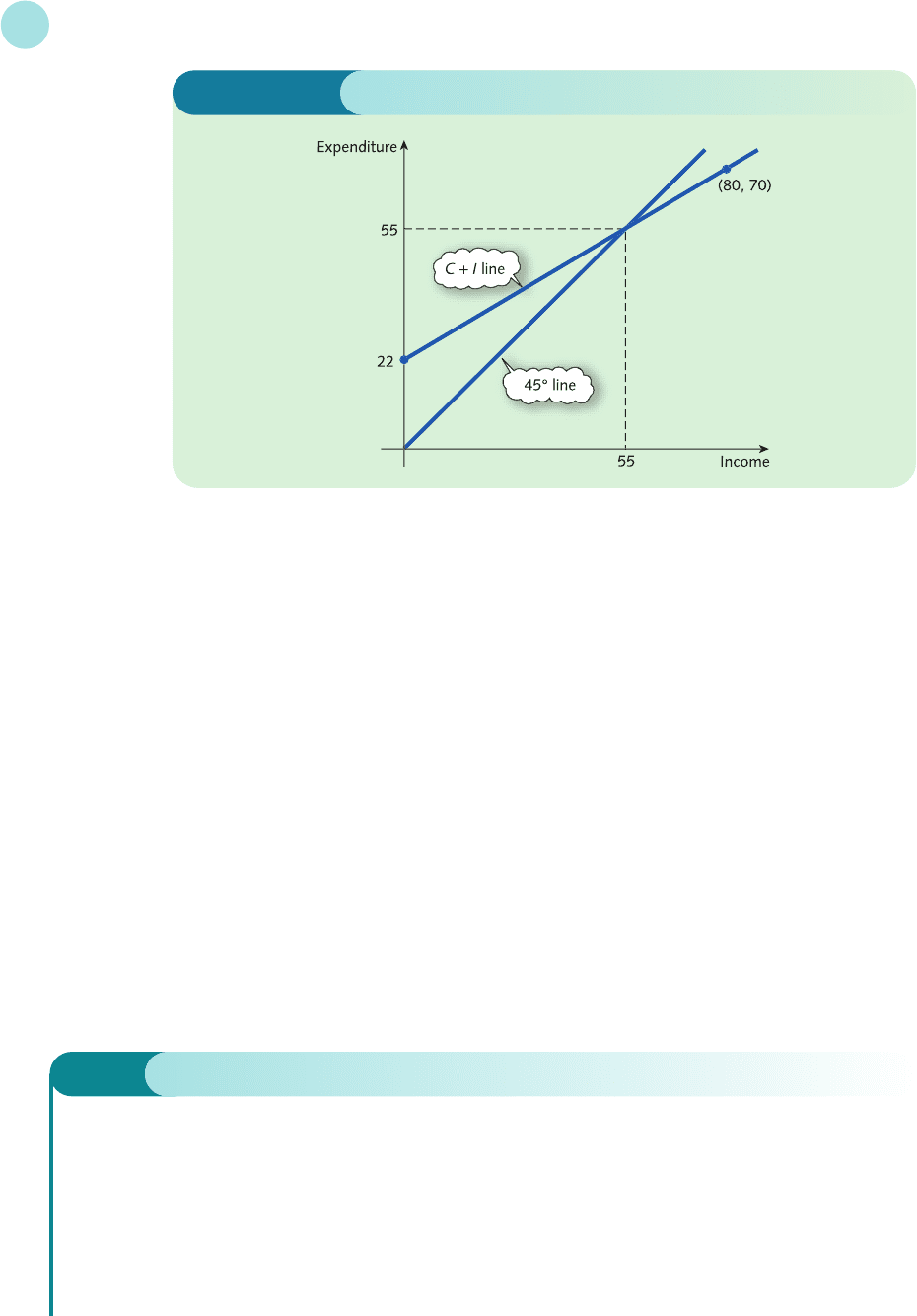
The equilibrium income can also be found graphically by plotting expenditure against income. In this
example the aggregate expenditure, C + I, is given by 0.6Y + 22. This is sketched in Figure 1.28 using the fact
that it passes through (0, 22) and (80, 70). Also sketched is the ‘45° line’, so called because it makes an angle
of 45° with the horizontal. This line passes through the points (0, 0), (1, 1),..., (50, 50) and so on. In other
words, at any point on this line expenditure and income are in balance. The equilibrium income can there-
fore be found by inspecting the point of intersection of this line and the aggregate expenditure line, C + I.
From Figure 1.28 this occurs when Y = 55, which is in agreement with the calculated value.
Practice Problem
2 Find the equilibrium level of income if the consumption function is
C = 0.8Y + 25
and planned investment I = 17. Calculate the new equilibrium income if planned investment rises by
1 unit.
MFE_C01f.qxd 16/12/2005 10:58 Page 101
Linear Equations
102
Y = C + I + G
We assume that planned government expenditure and planned investment are autonomous
with fixed values G* and I* respectively, so that in equilibrium
Y = C + I* + G*
The withdrawals box in Figure 1.27 now includes taxation. This means that the income that
households have to spend on consumer goods is no longer Y but rather Y − T (income less tax),
which is called disposable income, Y
d
. Hence
C = aY
d
+ b
with
Y
d
= Y − T
In practice, the tax will either be autonomous (T = T* for some lump sum T*) or be a propor-
tion of national income (T = tY for some proportion t), or a combination of both (T = tY + T*).
Figure 1.28
Example
Given that
G = 20
I = 35
C = 0.9Y
d
+ 70
T = 0.2Y + 25
calculate the equilibrium level of national income.
MFE_C01f.qxd 16/12/2005 10:58 Page 102

1.6 • National income determination
103
Solution
At first sight this problem looks rather forbidding, particularly since there are so many variables. However,
all we have to do is to write down the relevant equations and to substitute systematically one equation into
another until only Y is left.
We know that
Y = C + I + G (from theory) (1)
G = 20 (given in problem) (2)
I = 35 (given in problem) (3)
C = 0.9Y
d
+ 70 (given in problem) (4)
T = 0.2Y + 25 (given in problem) (5)
Y
d
= Y − T (from theory) (6)
This represents a system of six equations in six unknowns. The obvious thing to do is to put the fixed
values of G and I into equation (1) to get
Y = C + 35 + 20 = C + 55 (7)
This has at least removed G and I, so there are only three more variables (C, Y
d
and T) left to eliminate. We
can remove T by substituting equation (5) into (6) to get
Y
d
= Y − (0.2Y + 25)
= Y − 0.2Y − 25
= 0.8Y − 25 (8)
and then remove Y
d
by substituting equation (8) into (4) to get
C = 0.9(0.8Y − 25) + 70
= 0.72Y − 22.5 + 70
= 0.72Y + 47.5 (9)
We can eliminate C by substituting equation (9) into (7) to get
Y = C + 55
= 0.72Y + 47.5 + 55
= 0.72Y + 102.5
Finally, solving for Y gives
0.28Y = 102.5 (subtract 0.72Y from both sides)
Y = 366 (divide both sides by 0.28)
Practice Problem
3 Given that
G = 40
I = 55
C = 0.8Y
d
+ 25
T = 0.1Y + 10
calculate the equilibrium level of national income.
MFE_C01f.qxd 16/12/2005 10:58 Page 103

Linear Equations
104
To conclude this section we return to the simple two-sector model:
Y = C + I
C = aY + b
Previously, the investment, I, was taken to be constant. It is more realistic to assume that
planned investment depends on the rate of interest, r. As the interest rate rises, so investment
falls and we have a relationship
I = cr + d
where c < 0 and d > 0. Unfortunately, this model consists of three equations in the four
unknowns Y, C, I and r, so we cannot expect it to determine national income uniquely. The
best we can do is to eliminate C and I, say, and to set up an equation relating Y and r. This is
most easily understood by an example. Suppose that
C = 0.8Y + 100
I =−20r + 1000
We know that the commodity market is in equilibrium when
Y = C + I
Substitution of the given expressions for C and I into this equation gives
Y = (0.8Y + 100) + (−20r + 1000)
= 0.8Y − 20r + 1100
which rearranges as
0.2Y + 20r = 1100
This equation, relating national income, Y, and interest rate, r, is called the IS schedule.
We obviously need some additional information before we can pin down the values of Y
and r. This can be done by investigating
the equilibrium of the money market. The
money market is said to be in equilibrium
when the supply of money, M
S
, matches
the demand for money, M
D
: that is, when
M
S
= M
D
There are many ways of measuring the
money supply. In simple terms it can be
thought of as consisting of the notes and
coins in circulation, together with money
held in bank deposits. The level of M
S
is
assumed to be controlled by the central
bank and is taken to be autonomous,
so that
M
S
= M*
S
for some fixed value M*
S
.
The demand for money comes from
three sources: transactions, precautions and
speculations. The transactions demand is
used for the daily exchange of goods and
MFE_C01f.qxd 16/12/2005 10:58 Page 104

1.6 • National income determination
105
services, whereas the precautionary demand is used to fund any emergencies requiring unfore-
seen expenditure. Both are assumed to be proportional to national income. Consequently, we
lump these together and write
L
1
= k
1
Y
where L
1
denotes the aggregate transaction–precautionary demand and k
1
is a positive constant.
The speculative demand for money is used as a reserve fund in case individuals or firms decide
to invest in alternative assets such as government bonds. In Chapter 3 we show that, as inter-
est rates rise, speculative demand falls. We model this by writing
L
2
= k
2
r + k
3
where L
2
denotes speculative demand, k
2
is a negative constant and k
3
is a positive constant.
The total demand, M
D
, is the sum of the transaction–precautionary demand and speculative
demand: that is,
M
D
= L
1
+ L
2
= k
1
Y + k
2
r + k
3
If the money market is in equilibrium then
M
S
= M
D
that is,
M*
S
= k
1
Y + k
2
r + k
3
This equation, relating national income, Y, and interest rate, r, is called the LM schedule. If
we assume that equilibrium exists in both the commodity and money markets then the IS and
LM schedules provide a system of two equations in two unknowns, Y and r. These can easily be
solved either by elimination or by graphical methods.
Example
Determine the equilibrium income and interest rate given the following information about the commodity
market
C = 0.8Y + 100
I =−20r + 1000
and the money market
M
S
= 2375
L
1
= 0.1Y
L
2
=−25r + 2000
What effect would a decrease in the money supply have on the equilibrium levels of Y and r?
Solution
The IS schedule for these particular consumption and investment functions has already been obtained in
the preceding text. It was shown that the commodity market is in equilibrium when
0.2Y + 20r = 1100 (1)
MFE_C01f.qxd 16/12/2005 10:58 Page 105

Linear Equations
106
For the money market we see that the money supply is
M
S
= 2375
and that the total demand for money (that is, the sum of the transaction–precautionary demand, L
1
, and the
speculative demand, L
2
) is
M
D
= L
1
+ L
2
= 0.1Y − 25r + 2000
The money market is in equilibrium when
M
S
= M
D
that is,
2375 = 0.1Y − 25r + 2000
The LM schedule is therefore given by
0.1Y − 25r = 375 (2)
Equations (1) and (2) constitute a system of two equations for the two unknowns Y and r. The steps
described in Section 1.2 can be used to solve this system:
Step 1
Double equation (2) and subtract from equation (1) to get
0.2Y + 20r = 1100
0.2Y − 50r = 750 −
70r = 350 (3)
Step 2
Divide both sides of equation (3) by 70 to get
r = 5
Step 3
Substitute r = 5 into equation (1) to get
0.2Y + 100 = 1100
0.2Y = 1000 (subtract 100 from both sides)
Y = 5000 (divide both sides by 0.2)
Step 4
As a check, equation (2) gives
0.1(5000) − 25(5) = 375 ✓
The equilibrium levels of Y and r are therefore 5000 and 5 respectively.
To investigate what happens to Y and r as the money supply falls, we could just take a smaller value of
M
S
such as 2300 and repeat the calculations. However, it is more instructive to perform the investigation
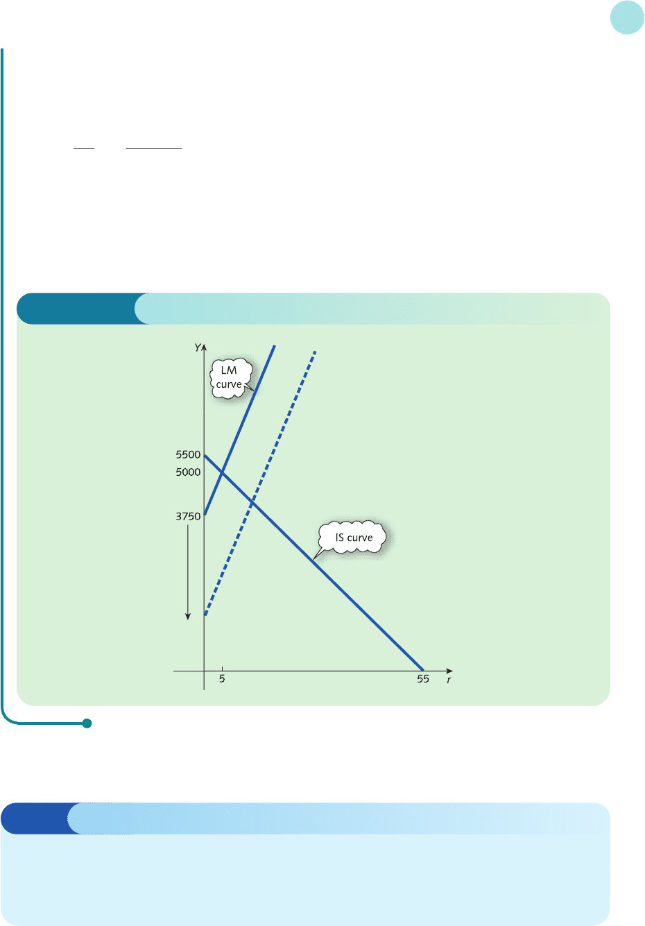
graphically. Figure 1.29 shows the IS and LM curves plotted on the same diagram with r on the horizontal
axis and Y on the vertical axis. These lines intersect at (5, 5000), confirming the equilibrium levels of inter-
est rate and income obtained by calculation. Any change in the money supply will obviously have no effect
on the IS curve. On the other hand, a change in the money supply does affect the LM curve. To see this, let
us return to the general LM schedule
MFE_C01f.qxd 16/12/2005 10:58 Page 106
1.6 • National income determination
107
k
1
Y + k
2
r + k
3
= M*
S
and transpose it to express Y in terms of r:
k
1
Y =−k
2
r − k
3
+ M*
S
(subtract k
2
r + k
3
from both sides)
Y = r + (divide both sides by k
1
)
Expressed in this form, we see that the LM schedule has slope −k
2
/k
1
and intercept (−k
3
+ M*
S
)/k
1
.
Any decrease in M*
S
therefore decreases the intercept (but not the slope) and the LM curve shifts down-
wards. This is indicated by the dashed line in Figure 1.29. The point of intersection shifts both downwards
and to the right. We deduce that, as the money supply falls, interest rates rise and national income decreases
(assuming that both the commodity and money markets remain in equilibrium).
−k
3
+ M*
S
k
1
D
F
−k
2
k
1
A
C
Advice
It is possible to produce general formulae for the equilibrium level of income in terms of
various parameters used to specify the model. As you might expect, the algebra is a little
harder but it does allow for a more general investigation into the effects of varying these
parameters. We will return to this in Section 5.3.
Figure 1.29
MFE_C01f.qxd 16/12/2005 10:58 Page 107

Linear Equations
108
Practice Problem
4 Determine the equilibrium income, Y, and interest rate, r, given the following information about the
commodity market
C = 0.7Y + 85
I =−50r + 1200
and the money market
M
S
= 500
L
1
= 0.2Y
L
2
=−40r + 230
Sketch the IS and LM curves on the same diagram. What effect would an increase in the value of
autonomous investment have on the equilibrium values of Y and r?
Example
(a) Given the consumption function
C = 800 + 0.9Y
and the investment function
I = 8000 − 800r
find an equation for the IS schedule.
(b) Given the money supply
M
S
= 28 500
and the demand for money
M
D
= 0.75Y − 1500r
find an equation for the LM schedule.
(c) By plotting the IS–LM diagram, find the equilibrium values of national income, Y, and interest rate, r.
If the autonomous investment increases by 1000, what effect will this have on the equilibrium position?
Solution
(a) The IS schedule is given by an equation relating national income, Y, and interest rate, r.
In equilibrium, Y = C + I. By substituting the equations given in (a) into this equilibrium equation,
we eliminate C and I, giving
Y = 800 + 0.9Y + 8000 − 800r
0.1Y = 8800 − 800r (subtract 0.9Y from both sides)
Y = 88 000 − 8000r (divide both sides by 0.1)
(b) The LM schedule is also given by an equation relating Y and r, but this time, it is derived from the equi-
librium of the money markets: that is, when M
S
= M
D
. Substituting the equations given in (b) into this
equilibrium equation gives
EXCEL
MFE_C01f.qxd 16/12/2005 10:58 Page 108
1.6 • National income determination
109
0.75Y − 1500r = 28 500
0.75Y = 28 500 + 1500r (add 1500r to both sides)
Y = 38 000 + 2000r (divide both sides by 0.75)
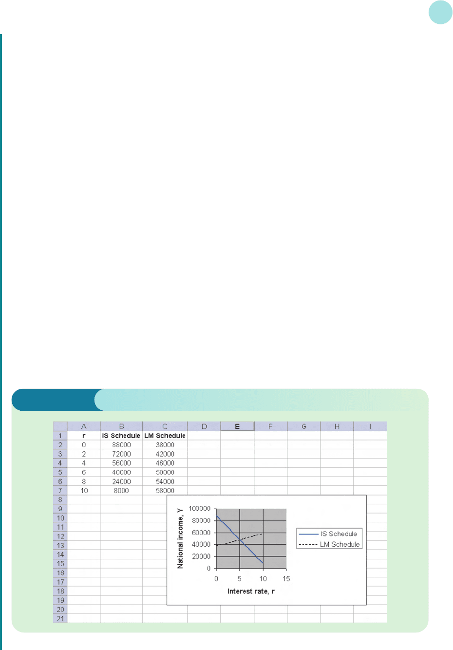
(c) To find the equilibrium position, we plot these two lines on a graph using Excel in the usual way. We
need to choose values for r and then work out corresponding values for Y. It is most likely that r will
lie somewhere between 0 and 10, so values of r are tabulated between 0 and 10, going up in steps of 2.
We type the formula
=88000−8000*A2
in cell B2 and type
=38000+2000*A2
in cell C2. The values of Y are then generated by clicking and dragging down the columns. Figure 1.30
shows the completed Excel screen.
Placing the cursor at the point of intersection tells us that the lines cross when
r = 5% and Y = 48 000
If the autonomous investment increases by 1000, the equation for the IS schedule will change, as the
equation for investment now becomes
I = 9000 − 800r
giving
Y = 98 000 − 8000r
The new IS schedule can be plotted on the same graph by adding a column of figures into the spread-
sheet, as shown in Figure 1.31.
Notice that the point of intersection has shifted both upwards and to the right. The equilibrium posi-
tion has now changed, resulting in a rise in interest rates to 6% and an increase in income to 50 000.
Figure 1.30
MFE_C01f.qxd 16/12/2005 10:58 Page 109