Jacques I. Mathematics for Economics and Business

Подождите немного. Документ загружается.

In Section 4.3 we described several applications of differentiation to economics. Starting

with any basic economic function, we can differentiate to obtain the corresponding marginal

function. Integration allows us to work backwards and to recover the original function from

any marginal function. For example, by integrating a marginal cost function the total cost func-

tion is found. Likewise, given a marginal revenue function, integration enables us to determine

the total revenue function, which in turn can be used to ﬁnd the demand function. These ideas

are illustrated in the following example, which also shows how the constant of integration can

be given a speciﬁc numerical value in economic problems.

Integration

430

Practice Problem

3 Find the indefinite integrals

(a)



(2x − 4x

)dx (b)



10x

+ dx (c)



(7x

− 3x + 2)dx

Example

(a) A ﬁrm’s marginal cost function is

MC = Q

+ 2Q + 4

Find the total cost function if the ﬁxed costs are 100.

(b) The marginal revenue function of a monopolistic producer is

MR = 10 − 4Q

Find the total revenue function and deduce the corresponding demand equation.

MPC = 0.5 +

and consumption is 85 when income is 100.

Solution

(a) We need to ﬁnd the total cost from the marginal cost function

MC = Q

+ 2Q + 4

Now

MC =

TC =



MCdQ



+ 2Q + 4)dQ

=+Q

+ 4Q + c

d(TC)

0.1

MFE_C06a.qxd 16/12/2005 11:22 Page 430

The ﬁxed costs are given to be 100. These are independent of the number of goods produced and repre-

sent the costs incurred when the ﬁrm does not produce any goods whatsoever. Putting Q = 0 into the

TC function gives

TC =+0

+ 4(0) + c = c

The constant of integration is therefore equal to the ﬁxed costs of production, so c = 100. Hence

TC =+Q

+ 4Q + 100

(b) We need to ﬁnd the total revenue from the marginal revenue function

MR = 10 − 4Q

Now

MR =

TR =



MRdQ



(10 − 4Q)dQ

= 10 − 2Q

+ c

Unlike in part (a) of this example we have not been given any additional information to help us to pin

down the value of c. We do know, however, that when the ﬁrm produces no goods the revenue is zero,

so that TR = 0 when Q = 0. Putting this condition into

TR = 10Q − 2Q

+ c

gives

0 = 10(0) − 2(0)

+ c = c

The constant of integration is therefore equal to zero. Hence

TR = 10Q − 2Q

Finally, we can deduce the demand equation from this. To ﬁnd an expression for total revenue from any

given demand equation we normally multiply by Q, because TR = PQ. This time we work backwards,

so we divide by Q to get

P == =10 − 2Q

so the demand equation is

P = 10 − 2Q

MPC = 0.5 +

Now

MPC =

0.1

10Q − 2Q

d(TR)

6.1 • Indefinite integration

431



MFE_C06a.qxd 16/12/2005 11:22 Page 431

C =



MRCdY



0.5 + dY

= 0.5Y + 0.2 Y + c

where the second term is found from



dY = 0.1



−1/ 2

dY = 0.1 Y

1/ 2

= 0.2 Y

The constant of integration can be calculated from the additional information that C = 85 when Y = 100.

Putting Y = 100 into the expression for C gives

85 = 0.5(100) + 0.2 100 + c = 52 + c

and so

c = 85 − 52 = 33

Hence

C = 0.5Y + 0.2 Y + 33

1/2

0.1

Integration

432

Practice Problem

4 (a) A firm’s marginal cost function is

MC = 2

Find an expression for the total cost function if the fixed costs are 500. Hence find the total cost

of producing 40 goods.

(b) The marginal revenue function of a monopolistic producer is

MR = 100 − 6Q

Find the total revenue function and deduce the corresponding demand equation.

MPS = 0.4 − 0.1Y

−1/ 2

and savings are zero when income is 100.

Example

A ﬁrm’s marginal revenue and marginal cost functions are given by

MR = 500 − 0.5Q

and MC = 140 + 0.4Q

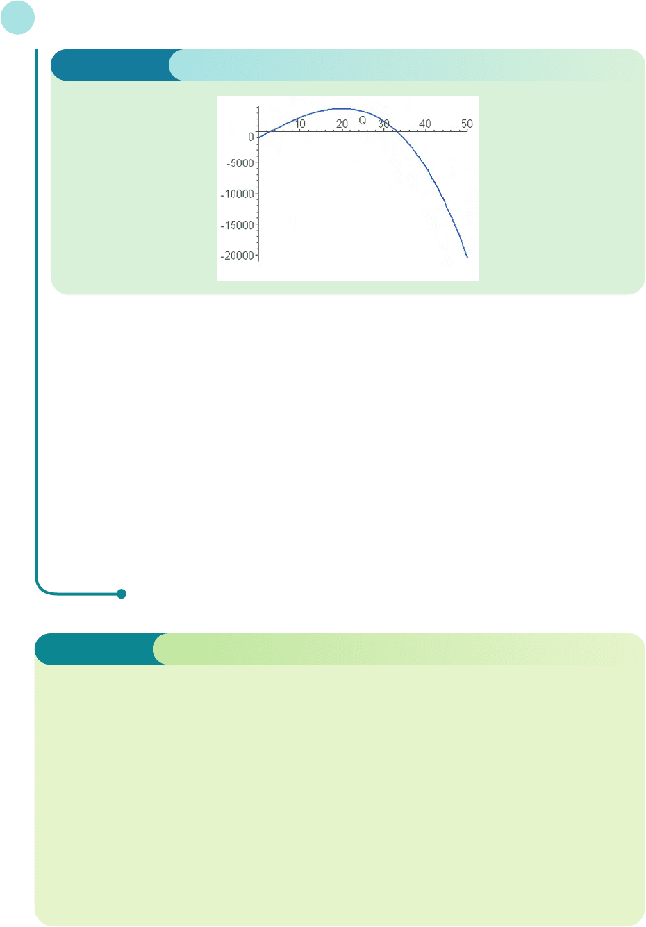
Given that total ﬁxed costs are 1000, plot a graph of the proﬁt function. Find the range of values of Q for

which the ﬁrm makes a proﬁt and ﬁnd its maximum value.

MAPLE

MFE_C06a.qxd 16/12/2005 11:22 Page 432

Solution

Let us begin by naming these two expressions as MR and MC by typing

>MR:=500-0.5*Q^2;

and

>MC:=140+0.4*Q^2;

Total revenue is the integral of marginal revenue and this is achieved by typing

>TR:=int(MR,Q);

which gives

TR:=500.Q-0.1666666667Q

Notice that Maple forgets to include the constant of integration! As it happens, the constant of integration

is zero in this case because TR = 0 when Q = 0. However, when we integrate MC we need to add on the ﬁxed

costs of 1000. We type

>TC:=int(MC,Q)+1000;

which gives

TC:=140.Q+0.1333333333Q

+1000

Proﬁt is then found by subtracting TC from TR so we type:

>profit:=TR-TC;

which gives

profit:=360.Q-.3000000000Q

–1000

In order to sketch a graph of the proﬁt function we need to specify the range of values of Q. Now total rev-

enue is deﬁned as PQ, so the demand equation can be found by dividing TR by Q to get

P = 500 − Q

This equation is valid only when P ≥ 0, i.e. when

500 − Q

≥ 0

This will be so provided

≤ 500 × 6 = 3000

so we require Q ≤ 3000 = 54.8.

If we now choose to sketch the graph between 0 and 50, we type

>plot(profit,Q=0..50);

which produces the diagram shown in Figure 6.1 (overleaf).

The ﬁrm makes a proﬁt when the graph lies above the horizontal axis. Figure 6.1 shows that this happens

between Q = 3 and Q = 33 approximately. The diagram also shows that the maximum proﬁt is roughly

$4000, which occurs when Q = 20.

If more precise values are required then these can easily be obtained by typing

>solve(profit=0,Q);

6.1 • Indefinite integration

433



MFE_C06a.qxd 16/12/2005 11:22 Page 433

which gives

–35.95428113, 2.795992680, 33.15828845

Only the positive solutions are relevant, so we deduce that the ﬁrm makes a proﬁt provided 2.8 ≤ Q ≤ 33.2.

Maximum proﬁt is achieved when MR = MC, so we type

solve(MR=MC,Q);

which gives

20., –20.

Again, the negative solution can be disregarded. The proﬁt itself is found by substituting Q = 20 into the

proﬁt function

>subs(Q=20,profit);

which gives $3800.

Integration

434

Anti-derivative A function whose derivative is a given function.

Constant of integration The arbitrary constant that appears in an expression when ﬁnding

an indeﬁnite integral.

Deﬁnite integration The process of ﬁnding the area under a graph by subtracting the

values obtained when the limits are substituted into the anti-derivative.

Indeﬁnite integration The process of obtaining an anti-derivative.

Integral The number ∫

f(x)dx (deﬁnite integral) or the function ∫f (x)dx (indeﬁnite

integral).

Integration The generic name for the evaluation of deﬁnite or indeﬁnite integrals.

Inverse The operation that reverses the effect of a given operation and takes you back to

the original. For example, the inverse of halving is doubling.

Primitive An alternative word for an anti-derivative.

Key Terms

Figure 6.1

MFE_C06a.qxd 16/12/2005 11:22 Page 434

6.1 • Indefinite integration

435

Practice Problems

5 Find

(a)



dx (b)



dx (c)



10e

10x

(d)



dx (e)



3/2

dx (f)



(2x

− 6x)dx

(g)



− 8x + 3)dx (h)



(ax + b)dx (i)



+ 4e

−2x

− dx

6 (1) Differentiate

F(x) = (2x + 1)

Hence find



(2x + 1)

(2) Use the approach suggested in part (1) to find

(a)



(3x − 2)

dx (b)



(2 − 4x)

(c)



(ax + b)

dx (n ≠−1) (d)



7 (a) Find the total cost if the marginal cost is

MC = Q + 5

and fixed costs are 20.

(b) Find the total cost if the marginal cost is

MC = 3e

0.5Q

and fixed costs are 10.

8 Find the total revenue and demand functions corresponding to each of the following marginal

revenue functions:

(a)

MR = 20 − 2Q (b) MR =

9 Find the consumption function if the marginal propensity to consume is 0.6 and consumption is 10

when income is 5. Deduce the corresponding savings function.

10 Find the short-run production functions corresponding to each of the following marginal product of

labour functions:

(a) 1000 − 3L

(b) − 0.01

11 (a) Show that

x( x + x

) = x + x

5/2

Hence find



x ( x + x

)dx

7x + 3



MFE_C06a.qxd 16/12/2005 11:22 Page 435

(b) Use the approach suggested in part (a) to integrate each of the following functions:

+ ,e

+ e

−x

+ 3), x

3/2

x −

12 (a) Show that

= x

− x + x

−1/ 2

Hence find



(b) Use the approach suggested in part (a) to integrate each of the following functions:

13 (Maple) If the marginal propensity to consume is given by

MPC =+

and C = 19/3 when Y = 4, find an expression for the consumption function. Plot both the consump-

tion function and the line C = Y on the same diagram. Use your graph to show that consumption

exceeds income for all values of Y in the range 0 < Y < k for some number k which should be stated.

14 (Maple)

(a) Find an expression for a firm’s short-run production function given that

= 10e

−0.02L

(50 − L)

(b) Find an expression for the total revenue function given that

MR =

100Q

1 + 50Q

2 Y

xxxx

−+

− e

−x

− x

+ x

− x

+ x

Integration

436

MFE_C06a.qxd 16/12/2005 11:22 Page 436

section 6.2

Definite integration

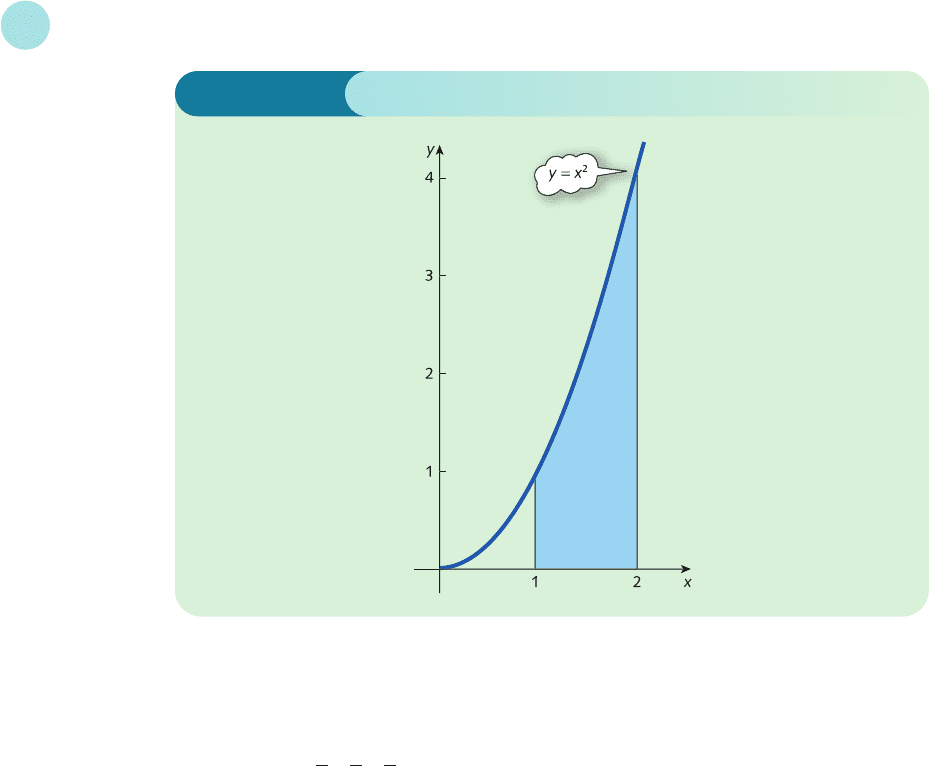
One rather tedious task that you may remember from school is that of ﬁnding areas. Sketched

in Figure 6.2 (overleaf) is a region bounded by the curve y = x

, the lines x = 1, x = 2, and the

x axis. At school you may well have been asked to ﬁnd the area of this region by ‘counting’

squares on graph paper. A much quicker and more accurate way of calculating this area is to

use integration. We begin by integrating the function

f(x) = x

to get

F(x) = x

In our case we want to ﬁnd the area under the curve between x = 1 and x = 2, so we evaluate

F(1) = (1)

F(2) = (2)

Objectives

At the end of this section you should be able to:

 Recognize the notation for deﬁnite integration.

 Evaluate deﬁnite integrals in simple cases.

 Calculate the consumer’s surplus.

 Calculate the producer’s surplus.

 Calculate the capital stock formation.

 Calculate the present value of a continuous revenue stream.

MFE_C06b.qxd 16/12/2005 11:21 Page 437

Finally, we subtract F(1) from F(2) to get

F(2) − F(1) =−=

This number is the exact value of the area of the region sketched in Figure 6.2. Given the con-

nection with integration, we write this area as



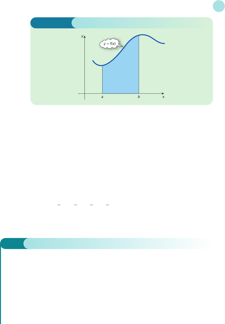
In general, the deﬁnite integral



f(x)dx

denotes the area under the graph of f(x) between x = a and x = b as shown in Figure 6.3. The

numbers a and b are called the limits of integration, and it is assumed throughout this section

that a < b and that f(x) ≥ 0 as indicated in Figure 6.3.

The technique of evaluating deﬁnite integrals is as follows. A function F(x) is found which

differentiates to f(x). Methods of obtaining F(x) have already been described in Section 6.1.

The new function, F(x), is then evaluated at the limits x = a and x = b to get F(a) and F(b).

Finally, the second number is subtracted from the ﬁrst to get the answer

F(b) − F(a)

In symbols,



f(x)dx = F(b) − F(a)

Integration

438

Figure 6.2

MFE_C06b.qxd 16/12/2005 11:21 Page 438

The process of evaluating a function at two distinct values of x and subtracting one from the

other occurs sufﬁciently frequently in mathematics to warrant a special notation. We write

[F(x)]

as an abbreviation for F(b) − F(a), so that deﬁnite integrals are evaluated as



f(x)dx = [F(x)]

= F(b) − F(a)

where F(x) is the indeﬁnite integral of f(x). Using this notation, the evaluation of



would be written as



dx = x

= (2)

− (1)

Note that it is not necessary to include the constant of integration, because it cancels out when

we subtract F(a) from F(b).

6.2 • Definite integration

439

Figure 6.3

Example

Evaluate the deﬁnite integrals

(a)



3dx (b)



(x + 1)dx

Solution

(a)



3dx = [3x]

= 3(6) − 3(2) = 12

This value can be conﬁrmed graphically. Figure 6.4 (overleaf) shows the region under the graph of

y = 3 between x = 2 and x = 6. This is a rectangle, so its area can be found from the formula

area = base × height



MFE_C06b.qxd 16/12/2005 11:21 Page 439