Jean-Laurent Mallet. Geomodeling
Подождите немного. Документ загружается.

568
CHAPTER
10.
DISCRETE
SMOOTH
PARTITION
the
values
of
this
function
are
close
to one
another; this
is
precisely
the
goal
of
the
next step.
•
Build
a
partition
of
{#1,...,
x
m
}
based
on the
attributes corresponding
to the
components
of
$(xi)
where
{</>i,
...,</>„}
are n <
m
points
in the
attributes' space
M
n
defined
by
the n
components
of
$(xi).
In
practice,
the
number
n of new
centers
{<^i,...,
<£>&}
should
be
chosen
to
have
the
same order
of
magnitude
as the
number
n of
output classes.
Let Ik be the set of
indexes
such
that
Using
the new
centers
{<^>i,...,
</>„}
denned
above,
we
propose
modifying
as fol-
lows
equation
(10.18)
to
extend
the
estimation
of the
conditional
Membership
Function
(p(e\X)
everywhere
on S for all j
e
{1,...,
n}:
About
the
output
The
above
estimation
method
can be
summarized
by the
following
expression:
For
each
input
value
X(e)
€
V(xi),
the
estimation
based
on the
Moving-
Centers
method
presented
above
generates
an
output
composed
of two
entities:
• the
centers
of
gravity
{yi,...,
y
n
}
of the
classes
{^i,...,
y
n
}
which
are
either
given
a
priori
or
built thanks
to the
Moving-Centers method;
• a
vector
<p(e\X]
whose components represent
the
probabilities
that
the
element
e
belongs
to the
classes
{^i,
• •
-,
3^n}
when
the
value
of
X(e)
is
already known
to
belong
to
V(xi).
These
results
can be
used
in a few
different ways,
depending
on the
nature
of
the
desired
output:
• To
obtain
a
unique output value
Y(e)
as an
answer
to the
input
X(e),
the
value
yj,
corresponding
to the
center
of the
most probable class,
may be
chosen:
• To
obtain
a set of
possible random values
for
Y(e),
it is
possible
to
proceed
as
follows:
—
draw
a
random
number
28
U(u)
uniformly
distributed
in the
range
[0,1],
28
As
usual,
<jj
is an
elementary
statistical
event
assumed
to
belong
to a set
13,
itself
part
of
a
Probabilized
Space
(U,A,
IP}.
10.4.
MOVING-CENTERS-BASED
METHODS
—
determine
the
index
j
such
that
—
select
at
random
a
value
Y(e,uj)
in the set
^.
As
can be
seen, proceeding
in
this
way
generates
a
random function
Y(e,u>)
defined
on
£.
•
Finally,
if the
elements
e
e
£ are
distributed
at the
nodes
of a
regular
N-grid,
then
the
Membership Function
ip(e\X)
can be
used
to
build
a
DSI
association
constraint (see section
(10.3.3)).
Analogy
with
neural
networks
As
suggested
in
figure
(10.13),
it is
relevant
to
note
that
there
is a
very
close
analogy
between
the
above
method
and the
notion
of
neural
network
used
for
solving
similar
problems
(e.g.,
see
[104]):
• the
centers
{xi,...,
x
m
}
are the
analog
of
the
nodes
of
the
"visible" input layer,
while
the
probabilities
\Xi
fl
3^|/|<-f;|
correspond
to the
associated
weightings;
• the
centers
{y\,...,
y
n
}
are the
analog
of the
nodes
of the
output layer;
• the
centers
{0i,...,0n}
are the
analog
of the
nodes
of the
"hidden" layer,
while
the
probabilities
|
Uie/
fe
Xi
H
J^|/|
Uie/
fc
Xi\
correspond
to the
associated
weightings;
• the
indicator functions
of the
Voronoi regions
{V(xi)}
and
{V((f)i)}
are the
analogs
of the
sigmoid
(logistic)
functions;
• the
construction
of the
centers
(0i,...,
0^}
and the
estimation
of the
proba-
bilities
|
Uj
€
/
fc
Xi
Pi
3^|/|
Uie/
fc
Xi\ are the
analog
of the
learning phase.
It
must
be
noted
that
the
proposed
method
has
some
advantages
as follows:
•
Compared
to the
so-called "back-propagation" algorithm used
in the
learning
phase
of
traditional neural networks,
the
Moving-Centers
algorithm
is
much
simpler
and
converges extremely
fast;
•
Compared
to the
obscure notions
of
weightings
and
sigmoid
functions
used
by
actual neural netwoks,
the
centers
{xi,...,
x
m
},
{0i,...,
0n},
and
{yi,...,
y
n
}
and
the
conditional probabilities
|
Uj
€
/
fc
Xi
fl
3^j|/|
Ui
£
/
fc
Xi\
have easily com-
prehensible physical interpretations;
•
Designing
the
architecture
of the
connections
of a net is
unnecessary, since
the
equivalent
is
realized automatically
by the
Moving-Centers method.
However,
in
spite
of its
analogy
with
neural
networks,
the
above
estimation
method
based
on the
Moving-Centers
cannot
be
considered
as a
regular
neural
network
technique.
For
this
reason,
we
suggest
using
the
acronym
"MC-
estimator"
to
designate
this
method.
569
570
CHAPTER
10.
DISCRETE SMOOTH PARTITION
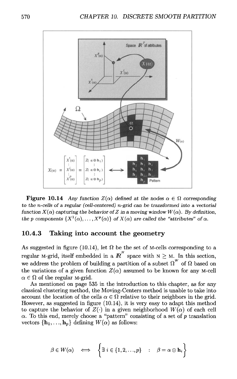
Figure
10.14
Any
function
Z(a)
defined
at the
nodes
a
e
f2
corresponding
to the
n-cells
of
a
regular
(cell-centered)
n-grid
can be
transformed
into
a
vectorial
function
X(o)
capturing
the
behavior
of
Z in a
moving
window
W(a).
By
definition,
the p
components
{X
v
(a),...,
X
p
(a)}
of
X(a)
are
called
the
"attributes"
of
a.
10.4.3 Taking into account
the
geometry
As
suggested
in
figure
(10.14),
let
Q
be the set of
M-cells
corresponding
to a
N
regular
M-grid,
itself embedded
in a
M
space with
N
>
M. In
this section,
W
we
address
the
problem
of
building
a
partition
of a
subset
f2
of 17
based
on
the
variations
of a
given
function
Z
(a]
assumed
to be
known
for any
M-cell
a
e
(7
of the
regular
M-grid.
As
mentioned
on
page
535 in the
introduction
to
this chapter,
as for any
classical clustering method,
the
Moving-Centers
method
is
unable
to
take into
account
the
location
of the
cells
a
G
0,
relative
to
their neighbors
in the
grid.
However,
as
suggested
in
figure
(10.14),
it is
very easy
to
adapt this method
to
capture
the
behavior
of
Z(-)
in a
given neighborhood
VF(o;)
of
each cell
a. To
this end, merely choose
a
"pattern" consisting
of a set of p
translation
vectors
{hi,..
.,h
p
}
denning
W(a)
as
follows:
10.4.
MOVING-CENTERS-BASED
METHODS
If
we let
then
the
Moving-Centers method
can be
used
to
build
a
series
of n
classes
W
{Ci,
• •
-i
C
n
}
corresponding
to a
partition
of
£1
:
W
In
this
case,
the
partition
of
0
so
obtained does actually
integrate
the ge-
ometry
of the
regular grid thanks
to the
moving window
W(a).
Note
that
this partitioning technique
is
easily adaptable
in the
case where
Z(a)
is not a
simple
function
but
rather
a
vectorial
function
with
q
compo-
nents
{Zi(oi),...,
Z
q
(a)}
defined
on
Q.
In
this case,
a
specific
window
Wj(a)
can be
associated
with each component
Zj(a),
and the
above definition (10.19)
can be
extended
as
follows:
with:
As
can be
seen,
the
dimension
p of the
resulting attributes' space
is
thus such
that
Proposal
for a
simulator
Let
us
assume
that
the
Moving-Centers-based method presented
in
section
(10.4.2)
is
used
for
estimating
a
parameter
Y(e)
=
Y(a)
in the
particular
case where
the
items
e
=
a are
distributed
on the
nodes
of a
regular grid.
In
this
case,
we can
think
of
slightly
modifying
the
algorithm presented
on
page
568
to
generate
a
random function
S(u(a),uj)
corresponding
to a
simulator
of
Y(a):
•
draw
an
event
u
belonging
to the
(abstract)
set
13
of all the
possible
events;
•
build
the
realization
P(u(a),
a;)
of a
P-field
honoring
a
given
covariance
func-
tion;
•
choose
the
index
j
such
that
•
select
at
random
a
value
S(u(a),uj)
in the set
3^-
Proceeding
in
this
way
allows
to
take into account
the
correlation between
Y(a)
and the
local behavior
of Z in
each neighborhood
W(a).
571
572
CHAPTER
10.
DISCRETE SMOOTH PARTITION
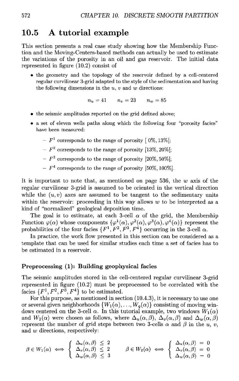
10.5
This
section presents
a
real case study showing
how the
Membership Func-
tion
and the
Moving-Centers-based methods
can
actually
be
used
to
estimate
the
variations
of the
porosity
in an oil and gas
reservoir.
The
initial
data
represented
in figure
(10.2)
consist
of
• the
geometry
and the
topology
of the
reservoir
defined
by a
cell-centered
regular curvilinear 3-grid
adapted
to the
style
of the
sedimentation
and
having
the
following
dimensions
in the
w,
v and w
directions:
• the
seismic
amplitudes
reported
on the
grid defined
above;
• a set of
eleven wells
paths
along which
the
following
four
"porosity
facies"
have been measured:
—
F
l
corresponds
to the
range
of
porosity
[ 0%,
13%[;
—
F
2
corresponds
to the
range
of
porosity
[13%,20%[;
—
F
3
corresponds
to the
range
of
porosity
[20%,50%[;
—
F
4
corresponds
to the
range
of
porosity
[50%,
100%].
It is
important
to
note
that,
as
mentioned
on
page 536,
the w
axis
of the
regular
curvilinear 3-grid
is
assumed
to be
oriented
in the
vertical direction
while
the
(u,v)
axes
are
assumed
to be
tangent
to the
sedimentary units
within
the
reservoir: proceeding
in
this
way
allows
w to be
interpreted
as a
kind
of
"normalized" geological deposition time.
The
goal
is to
estimate,
at
each
3-cell
a of the
grid,
the
Membership
Function
(p(a)
whose components
{(p
l
(a),
(p
2
(a},
(p
3
(a),
</?
4
(a)}
represent
the
probabilities
of the
four
facies
{-F
1
,
F
2
,
F
3
,
F
4
}
occurring
in the
3-cell
a.
In
practice,
the
work
flow
presented
in
this
section
can be
considered
as a
template
that
can be
used
for
similar studies each time
a set of
facies
has to
be
estimated
in a
reservoir.
Preprocessing
(1):
Building
geophysical
facies
The
seismic amplitudes stored
in the
cell-centered regular curvilinear 3-grid
represented
in figure
(10.2)
must
be
preprocessed
to be
correlated with
the
facies
{F
1
,
F
2
,
F
3
,
F
4
}
to be
estimated.
For
this purpose,
as
mentioned
in
section
(10.4.3),
it is
necessary
to use one
or
several given neighborhoods
{Wi(a;),...,
Wq(a)}
consisting
of
moving win-
dows
centered
on the
3-cell
a. In
this
tutorial example,
two
windows
Wi(a:)
and
W-2.(oi)
were chosen
as
follows,
where
A
u
(a,/3),
A
v
(o:,/:?)
and
A
w
(a,0)
represent
the
number
of
grid
steps
between
two
3-cells
a and (3 in the
u,
t>,
and w
directions, respectively:
10.5.
A
TUTORIAL EXAMPLE
573
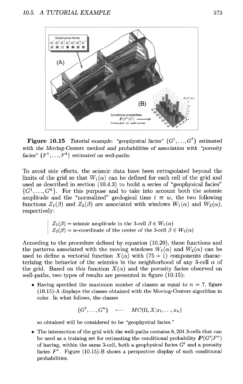
Figure
10.15
Tutorial example:
"geophysical
fades"
{G
l
,...,G
7
}
estimated
with
the
Moving-Centers
method
and
probabilities
of
association
with
"porosity
fades"
{F
1
,...,
F
4
}
estimated
on
well-paths.
To
avoid
side
effects,
the
seismic
data
have
been
extrapolated
beyond
the
limits
of the
grid
so
that
W\
(a) can be
defined
for
each
cell
of the
grid
and
used
as
described
in
section
(10.4.3)
to
build
a
series
of
"geophysical
fades"
{G
l
,...,G
n
}.
For
this
purpose
and to
take
into
account
both
the
seismic
amplitude
and the
"normalized"
geological
time
t
=
w,
the two
following
functions
Z\(fi]
and
Zi(fi)
are
associated
with
windows
W\(oi)
and
W^ot),
respectively:
Zi(fl)
=
seismic amplitude
in the
3-cell
/3
€
Wi(ct)
Z-i(&]
=
^-coordinate
of the
center
of the
3-cell
(3 E
W^ot)
According
to the
procedure
defined
by
equation
(10.20),
these
functions
and
the
patterns
associated
with
the
moving
windows
Wi(a)
and
W2(a)
can be
used
to
define
a
vectorial
function
X(a)
with
(75 + 1)
components
charac-
terizing
the
behavior
of the
seismics
in the
neighborhood
of any
3-cell
a of
the
grid.
Based
on
this
function
X(a)
and the
porosity
facies
observed
on
well-paths,
two
types
of
results
are
presented
in
figure
(10.15):
•
Having
specified
the
maximum number
of
classes
as
equal
to n = 7, figure
(10.15)-A
displays
the
classes obtained with
the
Moving-Centers algorithm
in
color.
In
what
follows,
the
classes
so
obtained
will
be
considered
to be
"geophysical facies."
• The
intersection
of the
grid with
the
well-paths contains
8, 204
3-cells
that
can
be
used
as a
training
set for
estimating
the
conditional probability
JP(G
1
\F
V
}
of
having, within
the
same 3-cell,
both
a
geophysical
facies
G
l
and a
porosity
facies
F
v
'.
Figure
(10.15)-B
shows
a
perspective display
of
such conditional
probabilities.
574
CHAPTER
10.
DISCRETE SMOOTH PARTITION
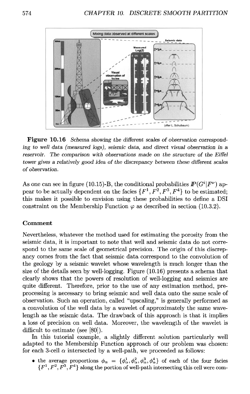
Figure
10.16
Schema
showing
the
different
scales
of
observation
correspond-
ing
to
well
data
(measured
logs),
seismic
data,
and
direct visual
observation
in a
reservoir.
The
comparison
with
observations
made
on the
structure
of the
Eiffel
tower
gives
a
relatively
good idea
of the
discrepancy
between
these
different
scales
of
observation.
As
one can see in
figure
(10.15)-B,
the
conditional probabilities
IP(G*
F
1
')
ap-
pear
to be
actually dependent
on the
facies
{F
1
,
F
2
,
F
3
,
F
4
}
to be
estimated;
this makes
it
possible
to
envision using these probabilities
to
define
a
DSI
constraint
on the
Membership
Function
(p
as
described
in
section (10.3.2).
Comment
Nevertheless,
whatever
the
method used
for
estimating
the
porosity
from
the
seismic
data,
it is
important
to
note
that
well
and
seismic
data
do not
corre-
spond
to the
same scale
of
geometrical precision.
The
origin
of
this discrep-
ancy comes
from
the
fact
that
seismic
data
correspond
to the
convolution
of
the
geology
by a
seismic wavelet whose wavelength
is
much longer
than
the
size
of the
details seen
by
well-logging. Figure (10.16) presents
a
schema
that
clearly
shows
that
the
powers
of
resolution
of
well-logging
and
seismics
are
quite
different.
Therefore,
prior
to the use of any
estimation method, pre-
processing
is
necessary
to
bring seismic
and
well
data
onto
the
same scale
of
observation. Such
an
operation, called
"upscaling,"
is
generally
performed
as
a
convolution
of the
well
data
by a
wavelet
of
approximately
the
same wave-
length
as the
seismic
data.
The
drawback
of
this approach
is
that
it
implies
a
loss
of
precision
on
well
data.
Moreover,
the
wavelength
of the
wavelet
is
difficult
to
estimate (see
[80]).
In
this tutorial example,
a
slightly
different
solution particularly
well
adapted
to the
Membership Function approach
of our
problem
was
chosen:
for
each
3-cell
a
intersected
by a
well-path,
we
proceeded
as
follows:
• the
average
proportions
^>
Q
=
{<$>&,
</>«>
</>a>
<^Q}
of
each
of the
four facies
{F
1
,
F
2
,
F
3
, F
4
}
along
the
portion
of
well-path
intersecting
this
cell were com-
10.5.
A
TUTORIAL
EXAMPLE
575
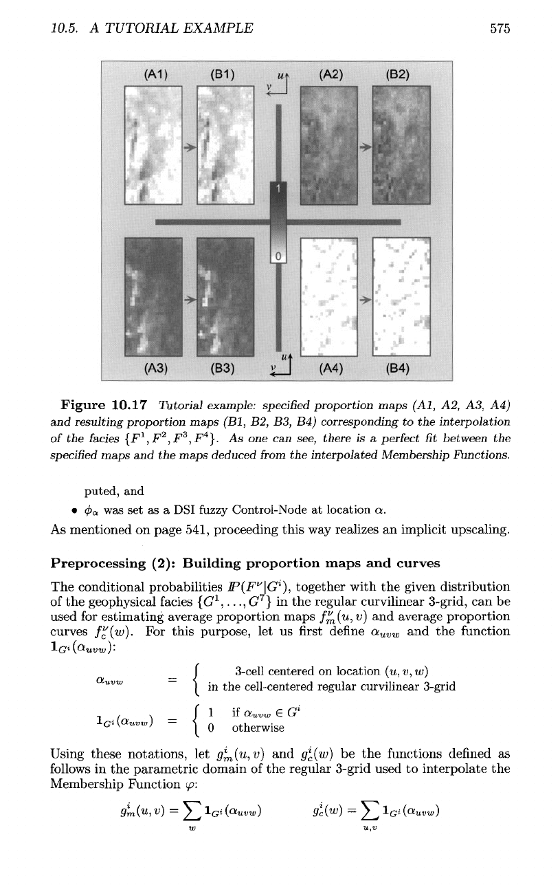
Figure
10.17
Tutorial example:
specified
proportion maps
(Al,
A2, A3, A4)
and
resulting proportion maps
(Bl,
B2, B3, B4)
corresponding
to the
interpolation
of
the
fades
{F
1
,
F
2
,
F
3
,
F
4
}.
As one can
see,
there
is a
perfect
fit
between
the
specified
maps
and the
maps
deduced
from
the
interpolated Membership Functions.
puted,
and
•
0
a
was set as a
DSI
fuzzy
Control-Node
at
location
a.
As
mentioned
on
page
541,
proceeding this
way
realizes
an
implicit
upscaling.
Preprocessing
(2):
Building proportion maps
and
curves
The
conditional probabilities
JP(F"|(7
Z
),
together with
the
given distribution
of
the
geophysical
facies
{G
1
,...,
G
7
} in the
regular curvilinear
3-grid,
can be
used
for
estimating average proportion maps
f^(u,v)
and
average proportion
curves
f"(w).
For
this purpose,
let us first
define
a
uvw
and the
function
^-G^^uvw)'-
_3-cell
centered
on
location
(w,
v,w)
~in the
cell-centered regular curvilinear 3-grid
_1
if
a
uvw
e
G
l
0
otherwise
Using
these
notations,
let
g
l
m
(u,v]
and
g
l
c
(w]
be the
functions defined
as
follows
in the
parametric domain
of
the
regular 3-grid used
to
interpolate
the
Membership
Function
(f>:
576
CHAPTER
10.
DISCRETE SMOOTH PARTITION
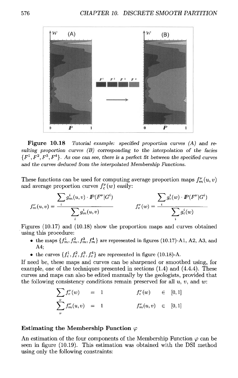
Figure
10.18
Tutorial example:
specified
proportion curves
(A) and re-
sulting proportion curves
(B)
corresponding
to the
interpolation
of the
fades
{F
1
,
F
2
,
F
3
,
.F
4
}.
As one can
see,
there
is a
perfect
fit
between
the
specified
curves
and
the
curves deduced
from
the
interpolated Membership Functions.
These
functions
can be
used
for
computing average proportion maps
/^(w,
v)
and
average proportion curves
fc(w)
easily:
Figures (10.17)
and
(10.18) show
the
proportion maps
and
curves obtained
using
this
procedure:
• the
maps
{/^,
/™,
/™,
/m}
are
represented
in
figures
(10.17)-A1,
A2, A3, and
A4;
• the
curves
{fc>fc,fc,fc}
are
represented
in figure
(10.18)-A.
If
need
be,
these maps
and
curves
can be
sharpened
or
smoothed using,
for
example,
one of the
techniques presented
in
sections (1.4)
and
(4.4.4).
These
curves
and
maps
can
also
be
edited
manually
by the
geologists, provided
that
the
following
consistency conditions remain preserved
for all
w,
i>,
and
w.
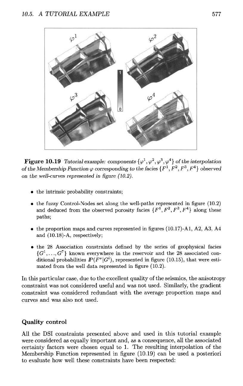
Estimating
the
Membership
Function
(f>
An
estimation
of the
four
components
of the
Membership Function
</?
can be
seen
in figure
(10.19). This estimation
was
obtained with
the
DSI
method
using
only
the following
constraints:
10.5.
A
TUTORIAL EXAMPLE
577
Figure
10.19
Tutorial example: components
{(f>
1
,
(f>
2
,
y?
3
,
<£>
4
}
of
the
interpolation
of
the
Membership Function
</?
corresponding
to the
fades
{F
1
,
F
2
,
F
3
,
F
4
}
observed
on
the
weJ]-curves
represented
in figure
(10.2).
• the
intrinsic probability constraints;
• the
fuzzy
Control-Nodes
set
along
the
well-paths represented
in figure
(10.2)
and
deduced
from
the
observed porosity
facies
{F
1
,
F
2
,
F
3
,
F
4
}
along these
paths;
• the
proportion maps
and
curves represented
in figures
(10.17)-A1,
A2, A3, A4
and
(10.18)-A,
respectively;
• the 28
Association constraints defined
by the
series
of
geophysical facies
{G
1
,...,^
7
}
known everywhere
in the
reservoir
and the 28
associated
con-
ditional probabilities
JP(F"|G
Z
),
represented
in figure
(10.15),
that
were
esti-
mated
from
the
well
data
represented
in figure
(10.2).
In
this particular case,
due to the
excellent quality
of the
seismics,
the
anisotropy
constraint
was not
considered
useful
and was not
used. Similarly,
the
gradient
constraint
was
considered redundant with
the
average proportion maps
and
curves
and was
also
not
used.
Quality
control
All
the
DSI
constraints presented above
and
used
in
this tutorial example
were
considered
as
equally important
and,
as a
consequence,
all the
associated
certainty factors
were
chosen equal
to 1. The
resulting interpolation
of the
Membership
Function represented
in
figure
(10.19)
can be
used
a
posteriori
to
evaluate
how
well
these constraints have been respected: