Johnson R.S. A Modern Introduction to the Mathematical Theory of Water Waves

Подождите немного. Документ загружается.

384 5 Epilogue

The removal of the viscous contribution involves U

-> 0 and 0t -> oo,

which clearly destroys the character of our KVB equation: we cannot

recover the KdV equation in the way we might have expected (but it does

arise if

let 0t -> 0). Nevertheless, we have succeeded in our intention

to find a limiting process that balances KdV nonlinearity and dispersion

against Burgers nonlinearity and dissipation.

The KVB equation, (5.75), possesses a number of interesting features.

First, it and our model admit a steady solution; second, the damping (or

dissipative) term

has a negative coefficient if

>f.

(5.76)

This condition implies an energy input and, presumably, we must antici-

pate that our model is no longer valid. In fact the speed of the surface

wave is, to leading order as e -> 0,

2UQ,

and all speeds have been non-

dimensionalised with respect to y^o^o* g

= gcosa; thus 2U

is the

Froude number of the wave. Thus, when we write F

—

, condition

(5.76) becomes

>\ or F>1.58.

Now it is commonly observed that bores with F larger than about 1.2

have turbulent, breaking fronts; on the other hand, if F is less than this

(but, of

course,

F > 1; see Section 2.7), we typically observe the undular

bore.

This suggests that our model has captured an important phenom-

enon (even though the values do not quite correspond); indeed, Dressier

(1949) has shown that the condition F

> 5/2 heralds the formation of

roll

waves, which, locally, have the appearance of turbulent bores.

This brie

f discussion of the role of laminar viscosity in water-wave

theory is brought to a close as we present a few observations on the

steady solutions of the KVB equation, (5.75). We seek a solution in the

form 7/

(£

—

cr), to give

-crjo

rjo

r]Q

—

- -

C/o)*7o

which, after one integration in f =

—

ex and imposing the condition

-> 0 as f

+oo, yields

Applications to the propagation of gravity waves 385

-cr/o

r,o

j (1

-1 ^

This equation is conveniently normalised by introducing the

transformation

to give

rjl -

+ i/o = ^o> (5.77)

where

In the form (5.77), we then have

770

-> 1 as f -> —00,

if solutions exist for which this is possible, which certainly requires

> 0

i.e. C/Q < 5/8. It is a

asymptotic behaviours

i.e.

C/Q

< 5/8. It is an elementary exercise (see Q5.15) to seek the

p(a£), f -• +00

and

~l-bexp(j8f), f -> -00,

and to find that

The choice

of the

sign

in a

ensures that

-> 0 as f ->

H-oo;

in ^,

either

sign

possible

(and it is

clear here that

must have

k > 0), but the

profile

as f ->

— 00

may be

either monotonic

(A > 2) or

oscillatory

< 2).

Thus equation (5.77) will allow either

monotonic transition

through

the

jump

non-turbulent classical jump)

or an

oscillation about

f7o

= l (th

undular bore).

The

interpretation

quite simply that larger

means larger dissipation (mainly

in the

neighbourhood

of f = 0), so no

wave

required

transport

the

excess energy away.

For

smaller

A, the

wave

needed

carry

the

surplus energy away from

the

front.

A number

interesting properties

of the

steady

KVB

equation

can be

explored

and

exploited;

see

Q5.16—Q5.19.

conclude

presenting

two

solutions

of the KVB

equation, (5.77),

Figure

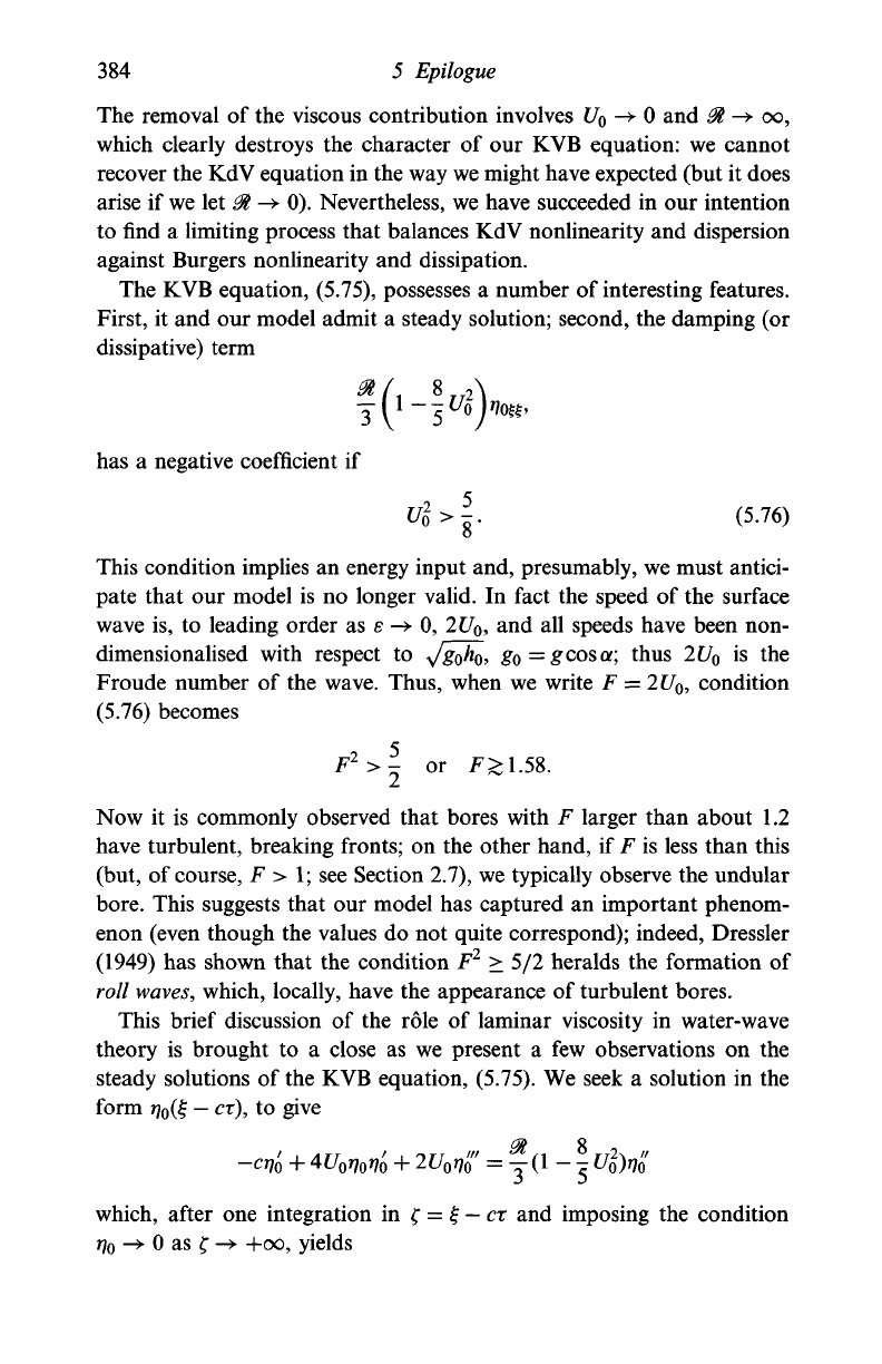
5.7;

these

are

based

386

-7.5

-5

-2.5 2.5 7.5

Figure 5.7. Two solutions of the steady state Korteweg-de Vries-Burgers (KVB)

equation, (5.77), for

0.1,

2.1.

numerical solutions of the equation. One is oscillatory (A = 0.1), and is

therefore a representation of the undular bore, and the other is a mono-

tonic profile (A = 2.1). The undular bore displays a front that is reminis-

cent of the solitary wave, and the oscillations can be described by an

evolving cnoidal wave; both these properties can be formalised by exam-

ining the limit

-> 0 (as considered in Johnson (1970)). The monotonic

profile, on the other hand, takes the form of

distorted

tank

curve, where

the distortion is progressively less pronounced as

-> oo; see Q5.18.

Further reading

The role of viscosity in fluid mechanics in general, and in the theory of

water waves in particular, is a very large and important subject. The

fundamental effects that are encountered in the study of fluids are best

addressed through standard texts on fluid mechanics (given, for example,

at the end of Chapter 1). However, in addition to the references already

given (including those relevant references contained therein), the reader is

directed to Lighthill (1978), Craik (1988) and Mei (1989) for some useful

Exercises 387

and fairly up-to-date material on viscous dissipation in wave propaga-

tion. The text by Debnath (1994) also touches on some of these ideas.

Exercises

Q5.1 Dispersion relation: large R. Consider the dispersion relation,

(5.21),

in the limit R -> oo at fixed 8k, and hence obtain result

(5.22):

(8k)

]

cosh

5/4

5A:sinh

3/4

5/cj'

Q5.2

Dispersion

relation:

8k = 0(1

/R).

Show that the result obtained

in Q5.1 is not uniformly valid, as 8k -* 0, where 8kR = O(l).

Hence obtain the equations that describe the leading approxima-

tion to the dispersion relation, (5.21), in the limit R -> oo at 8kR

fixed.

[Note: these equations cannot be solved in closed form.]

Q5.3

Dispersion

relation:

small 8k. Consider the dispersion relation,

(5.21),

in the limit 8k -> 0 at fixed R, and hence show that

~ -i8k

R/3

(where the real part of

turns out to be exponentially small).

[This case, which is essentially a high-viscosity limit, shows

that (at this order) there is no

propagation,

only decay. As an

additional exercise, you may show that the expression obtained

in Q5.2 agrees, for 8k -» oo, with that given in Q5.1 as 8k -» 0,

and that there is agreement between Q5.2 and Q5.3 for 8k -> 0.]

Q5.4

Dispersion

relation with surface

tension.

Repeat the calculation

presented in Section

5.2.1,

but with the surface pressure condi-

tion adjusted to accommodate the effects of surface tension,

namely

p — r\ w

—8

on z = 1;

cf. Section

2.1.

Hence obtain the dispersion relation, with surface

tension, which corresponds to that given in equation (5.21).

Q5.5 A model boundary layer problem. Obtain the solution of the

ordinary differential equation

388 5 Epilogue

that satisfies

where s > 0 is a constant. Describe the character of this solution,

for e -> 0, in the two cases

(a) x away from ;c = 0; (b) x = eX, X = O(l).

[The region near the boundary, measured by x = O(e) is where

the boundary layer exists; in this narrow region the solution

adjusts from the value e (approximately, as s -> 0) to 0 (on

* = 0).]

Q5.6 Asymptotic approach to a boundary layer problem. Solve the pro-

blem given in Q5.5 by seeking two asymptotic solutions, in the

form oo

(a) >>

valid for x away from x = 0, and satisfying the condition on

x=l;

(b) set x = sX and write

satisfying the condition on x = 0 (that is, onl = 0).

Now match the solutions obtained in (a) and (b), thereby

uniquely determining the solution in (b).

[You need find only the first terms in each expansion, but a

second could be found as well, if you are so minded.]

Q5.7 Inviscid solution of the viscous equations. Confirm that the solu-

tion given in equations (5.33) satisfies all the equations and

boundary conditions in (5.30)-(5.32), with the exception of the

no-slip condition on z = 0.

Q5.8 Surface shear-stress condition. Show that, away from the bound-

ary layer (formed as r^ 0), a solution exists in which

\zz +

Vog

= 0 (a term in equation (5.34)). Hence obtain an

expression for u^

and use this to confirm that the surface

shear-stress condition,

—

?7o£f

0 on z = 1,

is satisfied.

[This is the counterpart, at O(e), of the solution discussed in

Q5.7.]

Exercises 389

Q5.9 Heat I diffusion

equation:

Duhamel's

method.

The calculation of

the relevant solution of the equation

= u

> 0, x > 0,

is constructed in two stages.

(a) Obtain the solution for u(x, i) which satisfies

u(x, 0) = 0, x > 0;

w(0,

0 = 1. t > 0, (*)

in the form

U(x,

= l--j= j exp(-/)dj.

(b) The effect of raising the 'temperature' on x = 0 to

at a time

t = t' (> 0), and then reducing it to zero dXt = t' + h(h> 0),

is represented by the solution

U(x,

t-t')-

U(x, t-t

- h).

Over a very short time interval this is, approximately,

h(dU/dt) evaluated at time t

—

t'. If, during this interval,

the temperature is actually f(t\ the resulting temperature

over all times is then

this is Duhamel's result. Obtain an expression for dU/dt, and

hence write down

confirm that u = u is, indeed, a solution

of equation (*).

Hence rewrite this solution so that it takes the form quoted

in equation (5.42).

[In (a) introduce the similarity

variable,

x/2^~t. The solution

obtained in (b) gives the temperature (in x > 0, t > 0) when the

end, x = 0, is set at the variable temperature/(0- Here we have

used the interpretation of u as temperature, so (*) is called the

heat conduction equation in this context; it is also often called

the diffusion equation - here the diffusion of heat.]

390 5 Epilogue

Q5.10 An

integral

identity.

Show that

and evaluate this integral for the

choice/(JC)

= exp(—ax), where

a(> 0) is a real constant.

Q5.ll

Modulation

the

solitary

wave.

Follow the procedure described

in equation (5.49) et

seq.,

but start by multiplying this equation

Hence obtain the corresponding expression for c(T).

[This derivation uses the 'conserved' density

rjl,

rather than

as given in the text. You might wish to obtain numerical esti-

mates for the integrals that appear in these two formulae; the two

expressions for c(T) should, of course, be identical.]

Q5.12 Propagation of the modulated solitary wave. The

(nondimensional) speed of

the

solitary wave, in the characteristic

frame, is

where a (> 0) is a constant. Obtain an expression for the char-

acteristic variable (£) associated with the modulated solitary

wave; see equations (5.24).

Q5.13 Asymptotic

behaviour

the

bore.

Obtain an asymptotic solution

of the equation

(see equation (5.54)), in the form

ri~ae-

+ be-

\ x -> +oo.

Determine the relations between c, X, a, b and a, and compare

this behaviour with equation (2.165) et

seq.

and

Q2.63.

[The special case considered in Q5.10 will prove useful here.

Note that a and a could be related if the front of the wave were

to be like a solitary wave.]

Q5.14

Undular

bore:

perturbation pressure

O(e).

Obtain the pressure

term p

from equations (5.67)—(5.71), making use of the results

given in equations (5.72)-(5.74).

Exercises 391

Q5.15 Asymptotic

behaviours

the

KVB equation. Seek solutions of the

steady KVB equation

-rj + rj" = Xrj

(X > 0, constant)

in the forms

(a)

exp(-af), f -• +00;

(b) ij~l-&exp(j8?). ?"•-<»,

and hence determine a and jff.

Q5.16 Steady state KVB

equation:

phase plane

I. Discuss the equation

given in Q5.15 in the phase plane; that is, in the (rj,p) plane

where p = rj

. Show that there are two singular points, one at

(0,0) and the other at (1,0); determine their natures for various

X. In particular, include the cases:

= 0; 0 <

< 2.

Q5.17 Steady state KVB

equation: phase

plane

II. Repeat the calculation

of Q5.16, but this time write p = P/X and include the cases

1A = 0; X > 2.

Q5.18 KVB equation:

near-Taylor

profile.

Introduce the transformation

= XX into the equation in Q5.15, and hence obtain an

asymptotic solution in the form

[Asymptotic solutions can also be obtained for X -> 0

; see

Johnson (1970).]

Q5.19 KVB

equation:

special

solution.

Show that the steady state KVB

equation in Q5.15 has the exact solution

- tanh(f/2V6)} + \sech

(?/2V6),

when X = 5/V6.

Appendix A

The equations for a viscous fluid

The representation of a viscous fluid requires a change only to the form of the

local (short-range) force; the equation of mass conservation is unaltered. The

local force is now described through the (Cartesian) stress tensor,

(ij =1,2, 3), which represents the /-component of the stress (force/unit

area) on the surface whose outward normal is in

the y-direction.

If i =j then a^

is a

normal

stress,

and for i ^j it is a

tangential

shearing

stress.

In order

that the local forces give rise only to finite accelerations of a fluid particle, it is

necessary that ay be symmetric; that is, a

= a». Now, symmetric tensors

possess the property that, in a certain coordinate system (the

principal

coordinates

axes),

they may be written with diagonal elements only. (Indeed,

as the coordinates are transformed under rotations, the sum of the diagonal

elements is unchanged.) All this leads to the choice of stress tensor for a fluid

= -P8

j + d^

where P is the pressure in the fluid and 8

is the

Kronecker

delta;

dy is called

the

deviatoric stress tensor

and it is absent for a stationary fluid. It is this

contribution which is ignored in the derivation of Euler's equation, (1.12).

It is well established empirically (and supported by arguments based on

molecular transport) that, for most common fluids, d

is proportional to the

velocity gradients at a point in the fluid. Thus we write

where

ijk

is a rank four Cartesian tensor, and the

summation convention

employed; the position vector is written as x = (x\, x

, x

) and the

corresponding velocity vector is u = (u\, u

M3).

We require

to be symmetric

(because

is) and, further, we assume that the fluid is

isotropic;

that is, the

properties are the same in all directions. These considerations lead to

y y

where

6ij

" 2 \dxj ' dx

393