King M.R., Mody N.A. Numerical and Statistical Methods for Bioengineering: Applications in MATLAB
Подождите немного. Документ загружается.

then, since we can write
u ¼ 2v
1
v
2
;
u can be expressed as a linear combination of vectors v
1
and v
2
.
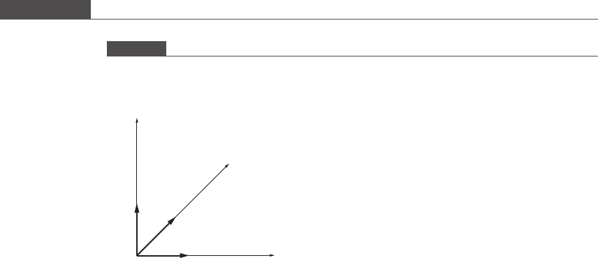
As another example, in three-dimensional space, every vector can be written as a
linear combination of the mutually perpendicular orthonormal vectors (see
Figure 2.4):
i ¼
1
0
0
2
4
3
5
; j ¼
0
1
0
2
4
3
5
; k ¼
0
0
1
2
4
3
5
;
such as
a ¼ 4i 3j þ 7k; b ¼ i þ k; c ¼ 2i þ j:
In fact, the matrix–vector multiplication operation Ax involves a linear com-
bination of the matrix column vectors to produce another column vector b.Ifa
matrix A is written as a series of column vectors, then the following demon-
strates how the transformation of the (n × 1) vector x by the (m × n) matrix A
can be viewed as an operation involving a linear co mbination of the matrix
columns:
b ¼ Ax ¼
a
11
a
12
a
13
... a
1n
a
21
a
22
a
23
... a
2n
:
:
:
a
m1
a
m2
a
m3
... a
mn
2
6
6
6
6
6
6
4
3
7
7
7
7
7
7
5
x
1
x
2
:
:
:
x
n
2
6
6
6
6
6
6
4
3
7
7
7
7
7
7
5
¼ a
1
a
2
... a
n
½
x
1
x
2
:
:
:
x
n
2
6
6
6
6
6
6
4
3
7
7
7
7
7
7
5
;
or
b ¼ x
1
a
1
þ x
2
a
2
þþx
n
a
n
;
or
Figure 2.4
Three-dimensional rectilinear coordinate system and the unit vectors (length or norm = 1) i, j, and k along the x-, y-,
and z-axes. This coordinate system defines our three-dimensional physical space.
x
y
z
i
j
k
Unit vectors along the x-, y-, and z-axes
67
2.2 Fundamentals of linear algebra

b ¼ x
1
a
11
a
21
:
:
:
a
m1
2
6
6
6
6
6
6
4
3
7
7
7
7
7
7
5
þ x
2
a
12
a
22
:
:
:
a
m2
2
6
6
6
6
6
6
4
3
7
7
7
7
7
7
5
þþx
n
a
1n
a
2n
:
:
:
a
mn
2
6
6
6
6
6
6
4
3
7
7
7
7
7
7
5
;
where
a
i
¼
a
1i
a
2i
:
:
:
a
mi
2
6
6
6
6
6
6
4
3
7
7
7
7
7
7
5
for 1 i n;
and b is another column vector of size m × 1.
In order for a vector u to be a linear combination of the vectors in set V, i.e.
u ¼ k
1
v
1
þ k
2
v
2
þþk
n
v
n
;
it is necessary that at least one non-zero scalar k
i
for 1 ≤ i ≤ n exists. If u cannot be
constructed from the vectors contained in the vector set V, then no combination
exists of one or more vectors in the set that can produce u. In other words, there are
no non-zero values for the scalar multipliers that permit u to be expressed as a linear
combination of vectors v
1
; v
2
; ...; v
n
.
Now let’s explore the properties of the vectors in the set V. Within a set of
vectors V = ðv
1
; v
2
; ...; v
n
Þ, it may be possible that we can express one or more
vectors as a linear combination of the other vectors in the set. We can write the
vector equation
k
1
v
1
þ k
2
v
2
þþk
n
v
n
¼ 0;
where again k
i
for 1 ≤ i ≤ n are scalars. The values of the scalar quantities for which
this equation holds true determine whether a vector in the set can be expressed as a
linear combination of one or more of the other vectors in the same set.
*
If one or more scalars in this equation can take on non-zero values, then we say that
the vectors in the set V are linearly dependent, i.e. a linear combination of one or
more vectors in the set can produce another vector in the same set.
*
If this equation holds true only when all k
i
= 0 for 1 ≤ i ≤ n, then the set of vectors
is said to be linearly independent. In other words, none of the vectors in the set
can be expressed as a linear combination of any of the other vector s in the same
set.
For example, the mutually perpendicular orthonormal vectors:
i ¼
1
0
0
2
4
3
5
; j ¼
0
1
0
2
4
3
5
; k ¼
0
0
1
2
4
3
5
are linearly independent. If we write the equation
k
1
i þ k
2
j þ k
3
k ¼ 0;
we obtain
68
Systems of linear equations

k
1
k
2
k
3
2
4
3
5
¼ 0;
which is valid only for k
1
= k
2
= k
3
=0.
2.2.5 Vector spaces and basis vectors
The space S that contai ns the set of vectors V and includes all vectors that result from
vector addition and scalar multiplication operations on the set V, i.e. all possible
linear combinations of the vectors in V is called a vector space.Ifu and v are two
vectors, and if W is a real vector space containing u and v, then W must also contai n
pu + qv , where p and q are any real scalar quantities. Commutative and associative
properties of vector addition and subtraction as well as scalar multiplication must
also hold in any vector space.
If the set of vectors V¼ðv
1
; v
2
; ...; v
n
Þ and all linear combinations of the vectors
contained in V completely define the size and extent of the vector space S, then S is
said to be spanned by the set of vectors V. For example, the set of vectors
i ¼
1
0
0
2
4
3
5
; j ¼
0
1
0
2
4
3
5
; k ¼
0
0
1
2
4
3
5
span the three-dimensional real space (R
3
).
If the vectors contained in set V are linearly independent,andifV spans a vector space
S,thenthesetofvectorsV is called a basis for the vector space S, and the individual
vectors in V are called basis vectors of S. There can be many basis sets for any vector
space S; however, all basis sets for the vector space S contain the same number of
linearly independent vectors. The number of vectors in a basis set determines the
dimension of the vector space S.Iftherearen vectors in a basis set V for vector space
S, then the dimension of the vector space is n.AnysetofvectorsthatspanS of
dimension n and has more than n vectors must be a linearly dependent set of vectors.
If R is the set of real numbers, then R
n
is a real space of dimension n and has n vectors in
any of its basis sets. For example, R
3
represents the three-dimensional physical space
that we live in, and an example of a basis vector set for this vector space is V =(i, j, k).
A matrix A of size m × n has a set of n column vectors:
A ¼
a
11
a
12
a
13
... a
1n
a
21
a
22
a
23
... a
2n
:
:
:
a
m1
a
m2
a
m3
... a
mn
2
6
6
6
6
6
6
4
3
7
7
7
7
7
7
5
¼ a
1
a
2
... a
n
½;
where
a
i
¼
a
1i
a
2i
:
:
:
a
mi
2
6
6
6
6
6
6
4
3
7
7
7
7
7
7
5
for 1 i n:
69
2.2 Fundamentals of linear algebra

The vector space spanned by the n column vectors is called the column space of A.If
the column vectors are linearly independent, then the dimension of the column space
of A is n. If the column vectors are linearly dependent on one another, i.e. at least one
column vector can be expressed in terms of a linear combination of one or more other
column vectors, then the dimension of the column space is <n. (The vector space
spanned by the m row vectors of the m × n matrix A is called the row space
3
of A.)
Example 2.1 Column space of a matrix
The 3 × 4 matrix
D ¼
1005
0108
0019
2
4
3
5
has four column vectors
d
1
¼
1
0
0
2
4
3
5
; d
2
¼
0
1
0
2
4
3
5
; d
3
¼
0
0
1
2
4
3
5
; and d
4
¼
5
8
9
2
4
3
5
:
The column space for this matrix is that vector space that is spanned by the four column vectors.
Each column vector can be expressed as a linear combination of the other three column vectors. For
example,
d
4
¼ 5d
1
þ 8d
2
þ 9d
3
and
d
1
¼
1
5
d
4
8d
2
9d
3
ðÞ:
Thus, the column vectors are linearly dependent. However, any vector set obtained by choosing three out
of the four column vectors can be shown to be linearly independent. The dimension of the column space of
D is therefore 3. In other words, a set of any three linearly independent vectors (each of size 3 × 1) can
completely define the column space of D.
Now that you are familiar with the concepts of column space of a matrix and linear
combination of vectors, we introduce the simple criterion for the existence of a
solution to a given set of linear equations Ax = b, where A is called the coefficient
matrix. The matrix–vector multiplication Ax, which forms the left-hand side of the
linear equations, produces a column vector b (right-hand side of the equations) that
is a linear combination of the column vectors of A.
A solution x to a set of linear equations Ax = b can be found if and only if the column vector b lies in the
column space of A, in which case the system of linear equations is said to be consistent. If the column
vector b does not lie in the column space of A (then b cannot be formed from a linear combination of the
column vectors of A), no solution to the system of linear equations exists, and the set of equations is
said to be inconsistent.
3
If the row vectors are linearly independent, then the dimension of the row space of A is m; otherwise, the
dimension of the row space is < m. For any matrix A, the row space and the column space will always
have the same dimension.
70
Systems of linear equations

2.2.6 Rank, determinant, and inverse of matrices
Matrix rank
The dimension of the column space of A (or equivalently the row space of A) is called the
rank of the matrix A. The rank of a matrix indicates the number of linearly independent
row vectors or number of linearly independent column vectors contained in the matrix.
It is always the case that the number of linearly independent column vectors equals the
number of linearly independent row vectors in any matrix. Since A has a set of n column
vectors and a set of m row vectors, if n > m the column vectors must be linearly
dependent. Similarly, if m > n the row vectors of the matrix must be linearly dependent.
The rank of an m × n matrix A is always less than or equal to the minimum of m and n.If
rank(A) < minimum of (m, n), then the column vectors form a linearly dependent set
andsodotherowvectors.SuchamatrixA is said to be rank deficient.
The rank of the coefficient matrix A is of primary importance in determining whether
a unique solution exists, infinitely many solutions exist, or no solution exists for a system
of linear equations Ax = b. The test for consistency of a system of linear equations
involves the construction of an augmented matrix [Ab], in which the column vector b is
added as an additional column to the right of the columns of the m × n coefficient matrix
A. The vertical dotted line in the matrix representation shown below separates the
coefficients a
ij
of the variables from the constants b
i
of the equations:
augmented matrix ! aug A ¼ A:b½
¼
a
11
a
12
a
13
... a
1n
: b
1
a
21
a
22
a
23
... a
2n
: b
2
: :
: :
: :
a
m1
a
m2
a
m3
... a
mn
: b
m
2
6
6
6
6
6
6
6
6
4
3
7
7
7
7
7
7
7
7
5
:
Consistency of the system of linear equations is guaranteed if rank(A) = rank(aug
A). Why? If the rank remains unchanged even after augmenting A with the column
vector b, then this ensures that the columns of aug A are linearly dependent, and thus
b lies wi thin the column space of A.InExample 2.1,ifD is an augmented matrix, i.e.
A ¼
100
010
001
2
4
3
5
; b ¼
5
8
9
2
4
3
5
; and D ¼½Ab;
then rank(A) = 3, rank(D) = 3, and the system of linear equations defined by D is
consistent.
If rank(aug A) > rank(A), then, necessarily, the number of linearly independent
columns in the augmented matrix is greater than that in A, and thus b cannot be
expressed as a linear combination of the column vectors of A and thus does not lie in
the column space of A.
For example, if
D ¼ Ab½¼
1005
0108
0009
2
4
3
5
71
2.2 Fundamentals of linear algebra

where
A ¼
100
010
000
2
4
3
5
; b ¼
5
8
9
2
4
3
5
;
you should show yourself that rank(A) ≠ rank(D). The system of equations defined
by D is inconsistent and has no solution.
The next question is: how does the rank of a matrix determine whether a unique
solution exists or infinitely many solutions exist for a consistent set of linear
equations?
*
If rank(A) = the number of column vectors n of the coefficient matrix A, then
the coefficient matrix has n linearly independent row vectors and column
vectors, which is also equal to the number of unknowns or the number of
elements in x. Thus, there exists a unique solution to the system of linear
equations.
*
If rank(A) < the number of column vectors n of the coefficient matrix A, then the
number of linearly independent row vectors (or column vectors) of A is less than the
number of unknowns in the set of linear equations. The linear problem is under-
defined, and there exist infinitely many solutions.
In summary, the test that determines the type of solution that a system of linear
equations will yield is defined below.
Unique solution:
(1) rank(A) = rank([Ab]), and
(2) rank(A) = number of column vectors of A.
Infinitely many solutions:
(1) rank(A) = rank([Ab]), and
(2) rank(A) < number of column vectors of A.
No solution:
(1) rank(A) < rank([Ab]).
In this chapter we are concerned with finding the solution for systems of equations
that are either
*
consistent and have a unique solution, or
*
inconsistent but overdetermined (or overspecified – a greater number of equations
than unknowns), i.e. rank(A)=n and m > n.
Using MATLAB
The rank function is provided by MATLAB to determine the rank of any matrix.
The use of rank is demonstrated below:
44
A = 2*ones(3,3) + diag([1 1], -1)
(Note that the second parameter in the diag function indicates the position of the
diagonal of interest, i.e. the main diagonal or diagonals below or above the main
diagonal.)
72
Systems of linear equations

A=
222
322
232
44
rank(A)
ans =
3
44
B=[102;264;346]
B=
102
264
346
44
rank(B)
ans =
2
Can you see why the matrix B does not have three linearly independent rows/columns?
Determinant of a matrix
The determinant is a scalar quantity that serves as a useful metric, and is defined for
square n × n matrices. The determinant of a matrix A is denoted by det(A)or A
jj
.
Note that Ajjis non-zero for square matrices A of rank = n and is zero for all square
matrices of rank < n. The determinant has properties that are different from its
corresponding matrix.
If A is an n × n matrix, then
A ¼
a
11
a
12
a
13
... a
1n
a
21
a
22
a
23
... a
2n
:
:
:
a
n1
a
n2
a
n3
... a
nn
2
6
6
6
6
6
6
4
3
7
7
7
7
7
7
5
;
and the determinant of A is written as
det AðÞ¼
a
11
a
12
a
13
... a
1n
a
21
a
22
a
23
... a
2n
:
:
:
a
n1
a
n2
a
n3
... a
nn
:
Note the diff erent styles of brackets used to distinguish a matrix from a determinant.
In order to calculate the determinant of a matrix, it is first necessary to know how
to calculate the cofactor of an element in a matrix. For any element a
ij
of matrix A,
the minor of a
ij
is denoted as M
ij
and is defined as the determinant of the submatrix
that is obtained by deleting from A the ith row and the jth column that contain a
ij
.
For example, the minor of a
11
is given by
M
11
¼
a
22
a
23
... a
2n
a
32
a
33
... a
3n
:
:
a
n2
a
n3
... a
nn
:
73
2.2 Fundamentals of linear algebra

The cofactor of a
ij
is defined as A
ij
=(−1)
i+j
M
ij
. The determinant of a matrix A
can be calculated using either of two formulas.
(1) Row-wise calculation of the determinant
A
jj
¼
X
n
j¼1
a
ij
A
ij
for any single choice of i 2 1; 2; ...; n
fg
: (2:13)
(2) Column-wise calculation of the determinant
A
jj
¼
X
n
i¼1
a
ij
A
ij
for any single choice of j 2 1; 2; ...; n
fg
: (2:14)
Note that the determinant of a single 1 × 1 matrix a
11
jj
¼ a
11
.
A2× 2 determinant is calculated by expanding along the first row:
a
11
a
12
a
21
a
22
¼ a
11
ja
22
a
12
jj
a
21
j¼a
11
a
22
a
12
a
21
:
Similarly, a 3 × 3 determinant is calculated by expanding along the first row:
a
11
a
12
a
13
a
21
a
22
a
23
a
31
a
32
a
33
¼ a
11
a
22
a
23
a
32
a
33
a
12
a
21
a
23
a
31
a
33
þ a
13
a
21
a
22
a
31
a
32
¼ a
11
a
22
a
33
a
23
a
32
ðÞa
12
a
21
a
33
a
23
a
31
ðÞ:
þ a
13
ða
21
a
32
a
22
a
31
Þ
If the determinant of a matrix is non-zero, the matrix is said to be non-singular;if
the determinant is zero, the matrix is said to be singular.
The calculation of determinants, especially for matrices of size n ≥ 4, is likely to
involve numerical errors involving scaling (overflow error) and round-off errors, and
requires a formidable numb er of computational steps. Expressing a matrix as a
product of diagonal or triangular matrices (LU factorization) enables faster and
simpler evaluation of the determinant and requires minimal number of computa-
tions. MATLAB provides the det function to calculate the determinant of a matrix.
Inverse of a matrix
Unlike matrix multiplication, matrix division is not formally defined. However,
inversion of a matrix is a well-defined procedure that is equivalent to matrix division.
Only square matrices that are non-singular (det(A) ≠ 0) can be inverted. Such matrices
are said to be invertible, and the inverted matrix A
1
is called the inverse of A.A
number divided by itself is equal to one. Similarly, if a matrix is multiplied by its
inverse, the identity matrix I is the result. Remember that the identity matrix is a
diagonal matrix that has ones on the diagonal and zeros everywhere else. Thus,
AA
1
¼ A
1
A ¼ I: (2:15)
It can be shown that only one inverse of an invertible matrix exists that satisfies
Equation (2.15). The method used to calculate the inverse of a matrix is derived from
first principles in many standard linear algebra textbooks (see, for instance, Davis
and Thomson (2000)) and is not discussed here. A brief demonstration of the method
used to calculate the inverse is shown in the following for a 3 × 3 square matrix A.If
74
Systems of linear equations

A ¼
a
11
a
12
a
13
a
21
a
22
a
23
a
31
a
32
a
33
2
4
3
5
then
A
1
¼
1
A
jj
A
11
A
21
A
31
A
12
A
22
A
32
A
13
A
23
A
33
2
4
3
5
; (2:16)
where A
ij
are cofactors of the elements of A. Note that the ijth element of the inverse
A
1
is equal to the cofactor of the jith element of A divided by the determinant of A.
MATLAB provides the inv function to calculate the inverse of a matrix.
For the matrix equation Ax = b, the solution x can be written as x = A
1
b, where
A
1
is the inverse of A. However, computation of the solution by calculating the
inverse is less efficient since it involves evaluating the determinant and requires many
more computational steps than solution techniques that are specially designed for
efficiently solving a system of linear equations. Some of these solution techniques
will be discussed in subsequent sections in this chapter.
An excellent introductory text on linear algebra by Anton (2004) is recommended
for further reading.
2.3 Matrix representation of a system of linear equations
A linear equation is defined as an equation that has a linear dependency on the
variables or unknowns in the equation. When the problem at hand involves more
than one variable, a system of coupled equations that describe the physical or
theoretical problem is formulated and solved simultaneously to obtain the solution.
If all the equations in the system are linear with respect to the n > 1 unknowns, then
we have a system of linear equations that can be solved using linear algebra theory. If
we have a system of n linear equations in n variables,
a
11
x
1
þ a
12
x
2
þ a
13
x
3
þþa
1n
x
n
¼ b
1
;
a
21
x
1
þ a
22
x
2
þ a
23
x
3
þþa
2n
x
n
¼ b
2
;
a
n1
x
1
þ a
n2
x
2
þ a
n3
x
3
þþa
nn
x
n
¼ b
n
;
then this system can be represented in the following compact form:
Ax ¼ b;
where
A ¼
a
11
a
12
a
13
... a
1n
a
21
a
22
a
23
... a
2n
:
:
:
a
n1
a
n2
a
n3
... a
nn
2
6
6
6
6
6
6
4
3
7
7
7
7
7
7
5
; x ¼
x
1
x
2
:
:
:
x
n
2
6
6
6
6
6
6
4
3
7
7
7
7
7
7
5
; and b ¼
b
1
b
2
:
:
:
b
n
2
6
6
6
6
6
6
4
3
7
7
7
7
7
7
5
:
75
2.3 Matrix representation of a set of linear equations

For this system of n equations to have a unique solution, it is necessary that the
determinant of A,|A| ≠ 0. If this is the case, the n × (n + 1) augmented matrix aug
A =[Ab] will have the same rank as that of A. The solution of a consistent set of n
linear equations in n unknowns is now reduced to a matrix problem that can be
solved using standard matrix man ipulation techniques prescribed by linear algebra.
Sections 2.4–2.6 discuss popular algebr aic techniques used to manipulate either A or
aug A to arrive at the desired solution. The pitfalls of using these solution techniques
in the event that A
jj
is close to zero are also explored in these sections.
2.4 Gaussian elimination with backward substitution
Gaussian elimination with backward substitution is a popular method used to solve
a system of equations that is consistent and has a coefficient matrix whose determi-
nant is non-zero. This method is a direct method. It involves a pre-defined number of
steps that only depends on the number of unknowns or variables in the equations.
Direct methods can be contrasted with iterative techniques, which require a set of
guess values to start the solution process and may converge upon a solution after a
number of iterations that is not known a priori and depends on the initial guess
values supplied. As the name implies, this solution method involves a two-part
procedure:
(1) Gaussian elimination , to reduce the set of linear equations to an upper triangular
format, and
(2) backward substitution, to solve for the unknowns by proceeding step-wise from the
last reduced equation to the first equation (i.e. “backwards”) and is suit able for a
system of equations in “upper” triangular form.
2.4.1 Gaussian elimination without pivoting
Example 2.2
The basic technique of Gaussian elimination with backward substitution can be illustrated by solving the
following set of three simultaneous linear equations numbered (E1)–(E3):
2x
1
4x
2
þ 3x
3
¼ 1; (E1)
x
1
þ 2x
2
3x
3
¼ 4; (E2)
3x
1
þ x
2
þ x
3
¼ 12: (E3)
Our first goal is to reduce the equations to a form that allows the formation of a quick and easy solution
for the unknowns. Gaussian elimination is a process that uses linear combinations of equations to
eliminate variables from equations. The theoretical basis behind this elimination method is that the solution
(x
1
; x
2
; x
3
) to the set of equations (E1), (E2), (E3) satisfies (E1), (E2) and (E3) individually and any linear
combinations of these equations, such as ( E2) – 0.5(E1)or(E3)+(E2).
Our first aim in this elimination process is to remove the term x
1
from (E2) and (E3) using (E1). If we
multiply (E1) with the constant 0.5 and subtract it from (E2), we obtain a new equation for (E2):
4x
2
4:5x
3
¼ 3:5: (E2
0
)
If we multiply (E1) with the constant 1.5 and subtract it from (E3), we obtain a new equation for (E3):
7x
2
3:5x
3
¼ 10:5 (E3
0
)
76
Systems of linear equations