Klir G.J. Uncertainity and Information. Foundations of Generalized Information Theory

Подождите немного. Документ загружается.

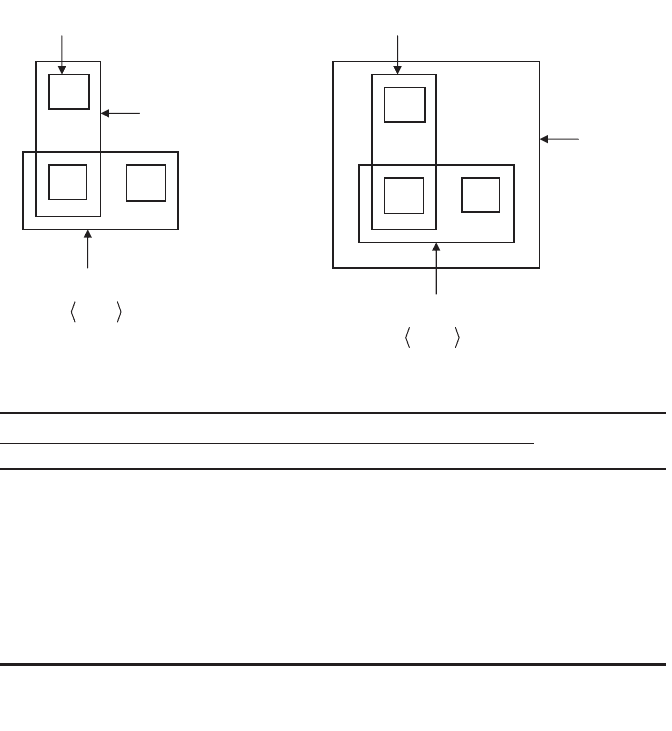
These bodies of evidence are also shown graphically in Figure 6.5a and 6.5b,

respectively.To determine whether ·F

, m

Ò£·F

, m

Ò, the three requirements,

(a)–(c), for ordering bodies of evidence in DST must be checked. Require-

ment (a) is trivially satisﬁed, since X ŒF

. Requirement (b) also satisﬁed for

, x

} ŒF

,{x

, x

} ŒF

; for {x

, x

} ŒF

,{x

} ŒF

; for X ŒF

, each set in F

sat-

isﬁes the condition. Requirement (c) is satisﬁed by constructing a function f

that satisﬁes Eqs. (6.31) and (6.32). For the given bodies of evidence, such a

function is shown in the table in Figure 6.5c. For clarity, all zero entries in the

table are left blank.

Using the introduced ordering of bodies of evidence in DST, the monoto-

nicity requirement for the GH measure can be stated as follows:

212 6. MEASURES OF UNCERTAINTY AND INFORMATION

∆ }{

x }{

x },{

xx },{

)(

0.2 0.2 0.6

)(

∆

}{

},{

0.5

}

0.5

0.1

}

0.1

f(A,B)

0.1 0.2 0.1 X 0.4

(c)

2.0})({

2.0}),({

211

xxm

6.0}),({

311

xxm

, m

(a)

1.0}),({

322

xxm

4.0)(

5.0}),({

312

xxm

, m

(b)

Figure 6.5. Illustrations of ordered bodies of evidence in DST (Example 6.5).

As is stated by the following theorem, the functional GH deﬁned by Eq. (6.27)

satisﬁes this monotonicity.

Theorem 6.4. For any pair of bodies of evidence in DST, ·F

, m

Ò and ·F

, m

Ò,

and for the functional GH deﬁned by Eq. (6.27),

(6.33)

Proof

䊏

6.3.3. Conditional Generalized Hartley Measures

The GH measure deﬁned by Eq. (6.27) is basically a weighted average of the

Hartley measure. Its conditional counterparts should thus be weighted aver-

ages of the respective conditional Hartley measures. It is thus meaningful to

deﬁne GH(X|Y) and GH(Y |X) by the formulas

(6.34)

(6.35)

where B 債 Y and A 債 X.

Now, Eq. (6.34) can be rewritten as

GH X Y m C C m C B

GH X Y m C B

GH X Y m B B

CXY CXY

CXY

CXYBY

()

=¥

()

=¥

()

=¥

()

Õ¥ Õ¥

Õ¥

Õ¥Õ

ÂÂ

log log

log

log .

GH Y X m C

CXY

()

Õ¥

log ,

GH X Y m C

CXY

()

Õ¥

log ,

mA A fAB A

fAB B

mB B

AX BABAX

BA BAX

AA BBX

12 2

()

ÕÕÕ

ÕÕ

ÂÂÂ

ÂÂ

log , log

, log

log .

11 22 1 2

,, .mmGHmGHm£ﬁ

()

if then FF

11 22 1 2

,,, .mmGHmGHm£

()

6.3. GENERALIZED HARTLEY MEASURE IN DEMPSTER–SHAFER THEORY 213

Hence,

(6.36)

and by a similar derivation,

(6.37)

These equations verify once more that the relationship among joint, marginal,

and conditional uncertainties is an invariant property of the uncertainty

theories.

6.4. GENERALIZED HARTLEY MEASURE FOR CONVEX SETS OF

PROBABILITY DISTRIBUTIONS

It is desirable to try to generalize the Hartley functional in DST to arbitrary

convex sets of probability distributions (credal sets). This generalized version

of the functional would be deﬁned by the formula

(6.38)

where D is a given set of probability distributions on X. Function m

in this

formula is obtained by the Möbius transformation applied to the lower prob-

ability function that is derived from D via Eq. (4.11).

It is easy to show that this functional GH is additive. That is,

(6.39)

when D is derived from D

and D

that are noninteractive, which means that

for all A ŒP(X) and all B Œ P(Y),

(6.40)

and m

this generalized case is virtually the same as the proof of additivity of GH in

DST (the proof of Theorem 6.3). Although values m

(A) in Eq. (6.38) may be

negative for some subsets of X, the equation

upon which the proof is based, still holds.

It is clear that the GH functional has the proper range, [0, log

|X|],

when the units of measurement are bits: 0 is obtained when D contains a single

()

mAB m Am B

DDD

()

◊

()

GH GH GH

XX YY

DD D

()

GH m A A

()

log ,

GH Y X GH X Y GH X

()

=¥

()

GH X Y GH X Y GH Y

()

=¥

()

214 6. MEASURES OF UNCERTAINTY AND INFORMATION

probability; log

|X| is obtained when D contains all possible probability

distributions on X, and thus represents total ignorance. The functional GH is

also continuous, symmetric (invariant with respect to permutations of the

probability distributions in D), and expansible (it does not change when com-

ponents with zero probabilities are added to the probability distributions

in D).

One additional property of the generalized Hartley functional, which is

signiﬁcant when we deal with credal sets, is its monotonicity with respect to

subsethood relationship between credal sets. This means that for every pair

of credal sets on X,

D and

D, if

D 債

D then GH(

D) £ GH(

D). This

property, whose proof is available in the literature (Note 6.6), is illustrated by

the following example.

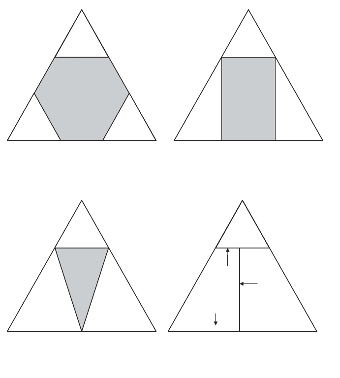
EXAMPLE 6.6. Consider six convex sets of probability distributions on X =

, x

} , which are denoted by

D(i Œ ⺞

) and are deﬁned geometrically

in Figure 6.6. Clearly,

D 傶

D and also

D 傶

D. However,

D is neither a subset nor a superset of any of the other sets. For each set

D(i Œ⺞

), the associated lower probability function,

–

its Möbius represen-

tation,

m, and the value GH(

D) of the GH measure are shown in Table 6.1.

In conformity with the monotonicity of GH,

and also GH(

D) ≥ GH(

D). Moreover, GH(

D) ≥ GH(

D) for all i Œ ⺞

which illustrates that nonspeciﬁcity GH(D) does not express the size of D.

While subadditivity of the generalized Hartley functional has been proven

for all uncertainty theories that are subsumed under DST (Theorem 6.2), the

following example demonstrates that the functional is not subadditive for arbi-

trary convex sets of probability distributions.

EXAMPLE 6.7. Let X = {x

, x

} and Y = {y

, y

} , and let z

=·x

, y

Ò for all i, j

Œ {1, 2} . Furthermore, let p =·p

, p

Ò denote joint probability distri-

butions on X ¥ Y, where p

= p(z

). Given the set D of all convex combina-

tions of probability distributions p

=·0.4, 0.4, 0.2, 0Ò and p

=·0.6, 0.2, 0, 0.2Ò,

we obtain the associated sets D

= {·0.8, 0.2Ò} and D

= {·0.6, 0.4Ò} of marginal

probability distributions. Clearly, GH(D

) + GH(D

) = 0. The lower proba-

bility function, m

–

associated with D and its Möbius representation, m

, are

shown in Table 6.2. Clearly, GH(D) = 0.332. Hence, GH is not subadditive in

this example.

It is easy to determine that the lower probability function m

–

in Example

6.7 is not 2-monotone. It contains eight violations of 2-monotonicity. One of

them is the violation of the inequality

mmmm

DDDD

zzz zz zz z

11 12 21 11 12 11 21 11

,, , , .

{}()

≥

{}()

GH GH GH GH

1234

DDDD

()

≥

()

≥

()

≥

()

6.4. GENERALIZED HARTLEY MEASURE FOR CONVEX SETS 215

Indeed, 0.8 ≥/ 0.8 + 0.6 - 0.4. Whether GH is subadditive or not for some less

general credal sets is an open question. However, this question looses its

signiﬁcance within the context discussed in Section 6.8.

6.5. GENERALIZED SHANNON MEASURE IN

DEMPSTER–SHAFER THEORY

The issue of how to generalize the Shannon entropy from probability theory

to DST has been discussed in the literature since the early 1980s. By and large,

216 6. MEASURES OF UNCERTAINTY AND INFORMATION

0.5, 0.5, 0

1/3, 0, 2/3 0, 1/3, 2/3 1/3, 0, 2/3 0, 1/3, 2/3

1/3, 2/3, 0 2/3, 1/3, 0

1/3, 0, 2/3 0, 1/3, 2/3

1, 0, 0

1, 0, 0 1, 0, 0 0, 1, 0 0, 1, 0

0, 1, 0

0, 0, 1 0, 0, 1

0, 0, 1

0, 2/3, 1/3

0, 1, 0 1/3, 2/3, 0 2/3, 1/3, 0 1, 0, 0

2/3, 0, 1/3

1/3, 0, 2/3 0, 1/3, 2/3

0, 0, 1

1/6, 1/6, 2/3

(a) (b)

(d)

0.5, 0.5, 0

(c)

Figure 6.6. Closed convex sets of probability distributions on X = {x

, x

} discussed in

Example 6.6.

Table 6.1 Lower Probability Functions and Their Möbius Representations for the Convex Sets of Probability Distributions on X = {x

, x

}

Deﬁned in Figure 6.6 and the Associated Values of the Generalized Hartley Measure GH (Example 6.6)

A:000000000 00000 0

100000000 1/61/6000 0

010000000 1/61/6000 0

001000000 002/32/30 0

1 1 0 1/3 1/3 1/3 1/3 1/3 1/3 1/3 0 1/3 1/3 1 1

1 0 1 1/3 1/3 1/3 1/3 0.5 0.5 0.5 1/3 2/3 0 0 0

0 1 1 1/3 1/3 1/3 1/3 0.5 0.5 0.5 1/3 2/3 0 0 0

11110101-1/310101 0

GH(

D) 1 1 0.805 2/3 1/3 1

217

the prospective generalized Shannon entropy was viewed in these discussions

as a measure of conﬂict among evidential claims in each given body of evi-

dence in DST. This view was inspired by the recognition that the Shannon

entropy itself is a measure of conﬂict associated with each given probability

distribution (recall the discussion of Eq. (3.25) in Chapter 3).

Although several intuitively promising functionals have been proposed as

candidates for the generalized Shannon entropy in DST, each of them was

found upon closer scrutiny to violate some of the essential requirements for

uncertainty measures. In most cases, it was the requirement of subadditivity,

perhaps the most fundamental requirement, that was violated. The efforts to

determine a justiﬁable generalization of the Shannon entropy in DST have

thus been unsuccessful.The reasons for this failure, which are now understood,

are explained later in this section.

Although none of the functionals proposed as a prospective generalization

of the Shannon entropy in DST is acceptable on mathematical grounds, it

seems useful to present their overview for at least two reasons: (1) ideas are

always better understood when we are familiar with the history of their devel-

opment; and (2) knowing which of the promising candidates have failed will

avoid their “reinventing.”

In the following overview of the unsuccessful attempts to generalize the

Shannon entropy to DST, no references are made.The relevant references are

all given in Note 6.7.

Two of the candidates for the generalized Shannon entropy in DST were

proposed in the early 1980s. One of them is functional E deﬁned by the

formula

218 6. MEASURES OF UNCERTAINTY AND INFORMATION

Table 6.2. Lower Probability Function m

in Examples 6.7 and 6.13

(A) m

(A)

A: 0 0 0 0 0.0 0.0

1 0 0 0 0.4 0.4

0 1 0 0 0.2 0.2

0 0 1 0 0.0 0.0

0 0 0 1 0.0 0.0

1 1 0 0 0.8 0.2

1 0 1 0 0.6 0.2

1 0 0 1 0.4 0.0

0 1 1 0 0.2 0.0

0 1 0 1 0.4 0.2

0 0 1 1 0.2 0.2

1 1 1 0 0.8 -0.2

1 1 0 1 0.8 -0.2

1 0 1 1 0.6 -0.2

0 1 1 1 0.4 -0.2

1 1 1 1 1.0 0.4

(6.41)

which is usually called a measure of dissonance. The other one is functional C

deﬁned by the formula

(6.42)

which is referred to as a measure of confusion. It is obvious that both of these

functionals collapse into the Shannon entropy when m deﬁnes a probability

measure.

To decide if either of the two functionals is an appropriate generalization

of the Shannon entropy in DST, we have to determine what these functionals

actually measure. From Eq. (5.47) and the general property of basic probabil-

ity assignments (satisﬁed for every A Œ P(X)),

(6.43)

we obtain

(6.44)

The term

in Eq. (6.44) represents the total evidential claim pertaining to focal elements

that are disjoint with the set A. That is, K(A) expresses the sum of all evi-

dential claims that fully conﬂict with the one focusing on the set A. Clearly,

K(A) Œ [0, 1]. The function

which is employed in Eq. (6.44), is monotonic increasing with K(A), and

extends its range from [0, 1] to [0, •). The choice of the logarithmic function

is motivated in the same way as in the classical case of the Shannon entropy.

It follows from these facts and the form of Eq. (6.44) that E(m) is the mean

(expected) value of the conﬂict among evidential claims within a given

body of evidence ·F, mÒ; it measures the conﬂict in bits and its range is

[0, log

|X|].

Functional E is not fully satisfactory since we feel intuitively that m(B) may

conﬂict with m(A) not only when B « A =∆. This broader view of conﬂict is

()

[]

log ,

1 KA

KA mB

()

«=∆

Em mA mB

ABA

()

«=∆Œ

ÂÂ

log .

mB mB

AB AB

()

«=∆ «π∆

ÂÂ

C m m A Bel A

()

() ()

log ,

E m m A Pl A

()

() ()

log ,

6.5. GENERALIZED SHANNON MEASURE IN DEMPSTER–SHAFER THEORY 219

expressed by the measure of confusion C given by Eq. (6.42). Let us demon-

strate this fact.

From Eq. (5.46) and the general property of basic assignments (satisﬁed for

every A ŒP(X)),

(6.45)

we get

(6.46)

The term

in Eq. (6.46) expresses the sum of all evidential claims that conﬂict with

the one focusing on the set A according to the following broader view of

conﬂict: m(B) conﬂicts with m(A) whenever B À

A. The reason for using the

function

instead of L(A) in Eq. (6.46) is the same as already explained in the context

of functional E. The conclusion is that C(m) is the mean (expected) value of

the conﬂict, viewed in the broader sense, among evidential claims within a

given body of evidence ·F, mÒ.

Functional C is also not fully satisfactory as a measure of conﬂicting

evidential claims within a body of evidence, but for a different reason than

functional E. Although it employs the broader, and more satisfactory, view

of conﬂict, it does not properly scale each particular conﬂict of m(B) with

respect to m(A) according to the degree of violation of the subsethood

relation B 債 A. It is clear that the more this subsethood relation is violated,

the greater the conﬂict. In addition, neither E nor C satisfy the essential

axiomatic requirement of subadditivity.

To overcome the deﬁciencies of functionals E and C as adequate measures

of conﬂict in evidence theory, a new functional, D, was proposed in the early

1990s:

(6.47)

Observe that the term

Dm mA mB

()

ŒŒ

ÂÂ

log .

()

[]

log

1 LA

LA mB

()

債

Cm mA mB

BAA

()

ÂÂ

log .

債

mB mB

BA BA

()

ÂÂ

債

220 6. MEASURES OF UNCERTAINTY AND INFORMATION

(6.48)

in Eq. (6.47) expresses the sum of individual conﬂicts of evidential claims with

respect to a particular set A, each of which is properly scaled by the degree to

which the subsethood B 債 A is violated. This conforms to the intuitive idea of

conﬂict that emerged from the critical reexamination of functionals E and C.

Clearly, Con(A) Œ [0, 1] and, furthermore,

(6.49)

The reason for using the function

instead of Con in Eq. (6.47) is exactly the same as previously explained in the

context of functional E. This monotonic transformation extends the range of

Con(A) from [0, 1] to [0, •).

Functional D, which is called a measure of discord, is clearly a measure of

the mean conﬂict (expressed by the logarithmic transformation of function

Con) among evidential claims within each given body of evidence. It follows

immediately from Eq. (6.49) that

(6.50)

Observe that |B - A|=|B|-|A « B| and, consequently, Eq. (6.47) can be

rewritten as

(6.51)

It is obvious that

(6.52)

Although functional D is intuitively more appealing than functionals E and

C, further examination revealed that it has a conceptual defect.To explain the

defect, let sets A and B in Eq. (6.47) be such that A Ã B. Then, according to

function Con, the claim m(B) is taken to be in conﬂict with the claim m(A) to

the degree |B - A|/|B|. This, however, should not be the case: the claim focus-

ing on B is implied by the claim focusing on A (since A Ã B) and, hence, m(B)

should not be viewed in this case as contributing to the conﬂict with m(A).

Consider, as an example, incomplete information regarding the age of a

person, say Joe. Assume that the information is expressed by two evidential

Bel A m B

Pl A

()

Dm mA mB

()

() ()

ŒŒ

ÂÂ

log .

Em Dm Cm

()

[]

log

1 Con A

K A Con A L A

()

Con A m B

()

6.5. GENERALIZED SHANNON MEASURE IN DEMPSTER–SHAFER THEORY 221