Koren B., Vuik K. (Editors) Advanced Computational Methods in Science and Engineering
Подождите немного. Документ загружается.

Hybrid N-S/DSMC Simulations of Gas Flows with Rarefied-Continuum Transitions
able Hard Sphere (VHS) [33] model, and the 2-parameter so-called Variable Soft
Sphere (VSS) [34, 35] model. With the first it is possible to accurately reproduce
the temperature dependence of the viscosity, whereas with a VSS model also the
temperature dependence of (thermal) diffusivities can be accounted for.
3.3.4 Sampling
Due to the relatively low number of computational particles (compared to the num-
ber of molecules in a physical system), DSMC results suffer from statistical noise.
The amount of noise is reduced by sampling the molecular properties during many
time steps (for a steady problem) or many ensembles (for an unsteady problem).
For steady state flow problems, sampling of the flow properties is performed inside
the time step loop and over many time steps once steady state has been reached.
Because two consecutive samples are usually highly correlated, sampling is usually
done once every ∼ 4 times steps. Flow properties are averaged over the same cells
as used for the collision routines. Within one cell and at one sampling time, the
following particle properties are accumulated:
• number of particles N,
• the sum of their velocities
∑
¯
V
i
,
• the sum of the square of their velocities
∑
(
¯
V ·
¯
V)
i
.
All relevant flow data such as the mass-average velocity
¯
V
ma
, the temperature T and
the density
ρ
can be calculated from these data. The density is calculated as:
ρ
= F
num
Nm
sV
. (62)
The equation for the mass-average velocity is:
¯
V
ma
=
∑
¯
V
i
N
. (63)
Finally, the temperature is determined as:
T =
m[
∑
(
¯
V ·
¯
V)
i
−
¯
V
ma
·
¯
V
ma
]
3k
B
. (64)
For unsteady flows, sampling during many time steps is not possible. In this case,
many ensembles are calculated, and the flow properties are derived by averaging
over all ensembles the samples taken at a specific time. This can be time and mem-
ory consuming due to the large number of ensembles which are needed and the
necessity of storing sample data also as a function of time.
417

G. Abbate, B.J. Thijsse, and C.R. Kleijn
3.4 Dynamic coupling of Navier-Stokes and DSMC solvers
3.4.1 Breakdown parameter
The first issue in developing a coupled N-S/DSMC method is how to determine
the appropriate computational domains for the DSMC and N-S solvers, and the
proper interface boundary between these two domains. The continuum breakdown
parameter Kn
max
[36] is employed in the present study as a criterion for selecting
the proper solver
Kn
max
= max[Kn
ρ
,Kn
V
,Kn
T
], (65)
where Kn
ρ
, Kn
V
and Kn
T
are the local Knudsen numbers based on density, velocity
and temperature length scales, according to
Kn
Q
=
λ
Q
ref
|▽Q|. (66)
Here, Q is a flow property (density, velocity or temperature) and
λ
is the local mean
free path length. Q
ref
is a reference value for Q, which can be either its local value
(for temperature or pressure), or a typical value (for the velocity). If the calculated
value of the continuum breakdown parameter Kn
max
in a region is larger than a lim-
iting value Kn
split
, then that region cannot be accurately modelled using the N-S
equations, and DSMC has to be used.
Two different strategies have been implemented for coupling the Navier-Stokes
based CFD code and the DSMC code: one for steady state flow simulations, the
other for unsteady flow simulations. Both will be described below.
3.4.2 Steady-state formulation
The proposed coupling method for steady flows is based on the Schwarz method
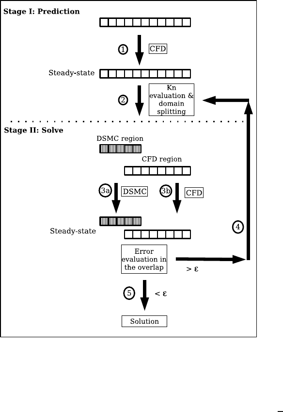
[17] and it consists of two stages (fig.2).
The first stage is a prediction stage, where the unsteady N-S equations are integrated
in time on the entire domain
Ω
until a steady state is reached. From this steady state
solution, the continuum breakdown parameter Kn
max
is computed and its values are
used to split
Ω
in the subdomains
Ω
DSMC
(Kn
max
> Kn
split
), where the flow field
will be evaluated using DSMC, and
Ω
CFD
(Kn
max
< Kn
split
), where the N-S equa-
tion will be solved. For Kn
split
a value of 0.05 was used. Between the DSMC and
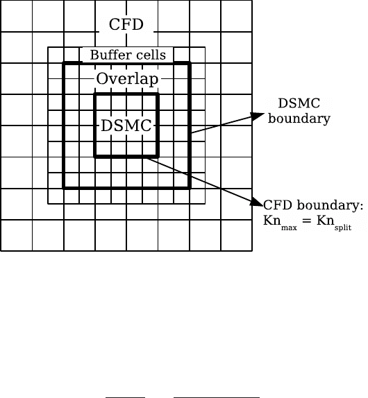
CFD regions an overlap region is considered, where the flow is computed with both
the DSMC and the CFD solver (fig.3).
In the second stage, DSMC and CFD are run in their respective subdomains with
their own time steps (
∆
t
DSMC
and
∆
t
CFD
, respectively), until a steady state is
reached.
First DSMC is applied; molecules are allocated in the DSMC subdomain, created
418
Hybrid N-S/DSMC Simulations of Gas Flows with Rarefied-Continuum Transitions
Fig. 2 Scheme of the coupling method for steady-state flows.
from a Chapman-Enskog velocity distribution, according to the density, velocity and
temperature obtained from the initial CFD solution. The grid is automatically refined
in the DSMC region in order to respect the DSMC requirements (
∆
x,
∆
y,
∆
z <
λ
3
).
The boundary conditions to the DSMC region come from the solution in the CFD
region. As described in the previous section 3.3.2 ”particle reservoir cells” are con-
sidered outside the overlapping region. In these cells molecules are created accord-
ing to the density, velocity, temperature and their gradients in the CFD solution with
a Chapmann-Enskog velocity distribution.
After running the DSMC, the N-S equations are solved in the CFD region. The
boundary conditions come from the solution in the DSMC region, averaged over
the CFD cells.
Once a steady state solution has been obtained in both the DSMC and N-S regions,
419
G. Abbate, B.J. Thijsse, and C.R. Kleijn
Fig. 3 Illustration of the Schwarz coupling method in a 2-D geometry.
the continuum breakdown parameter Kn
max
is re-evaluated and a new boundary be-
tween the two regions is computed. This second stage is iterated until in the over-
lapping region the relative difference between the DSMC and CFD solutions
∆
Q
Q
DSMC
=
Q
CFD
−Q
DSMC
Q
DSMC
, (67)
with Q a flow property (e.g. pressure or temperature), is less than a prescribed value
ε
(typically,
ε
≈ 0.001 [8]).
The advantage of using a Schwarz method with Dirichlet-Dirichlet boundary con-
ditions, instead of the more common Neumann-Neumann boundary conditions cou-
pling technique [19], is that the latter requires a much higher number of samples
than the Schwarz method [19]. In fact, the DSMC statistical scatter involved in de-
termining the fluxes is much higher than that associated with the macroscopic state
variables.
3.4.3 Unsteady formulation
In the unsteady formulation, the coupling method described above is re-iterated ev-
ery coupling time step
∆
t
coupling
≫
∆
t
DSMC
,
∆
t
CFD
, starting from the solution at the
previous time step.
During every coupling time step, the predicted DSMC region is compared to the one
of the previous time step. In the cells that still belong to the DSMC region, we con-
sider the same molecules of the previous time step, whose properties were recorded.
420
Hybrid N-S/DSMC Simulations of Gas Flows with Rarefied-Continuum Transitions
In these cells, it is important to consider the same molecules of the previous time
step rather than sampling them from continuum variables (temperature, density and
velocity) with a Maxwellian or a Chapman-Enskog velocity distribution. The use of
a Maxwellian or a Chapman-Enskog velocity distribution, in fact, presumes either
equilibrium or near-equilibrium conditions, which is not necessarily true in these
cells.
Molecules that are in the cells that no longer belong to the DSMC region are deleted.
In cells that have changed from being a CFD cell into a DSMC cell, new molecules
are created with a Chapmann-Enskog velocity distribution, according to the density,
velocity and temperature of the CFD solution at the previous time step.
At the end of every coupling step, molecule properties are recorded to set the initial
conditions in the DSMC region for the next coupling step.
4 Results and discussion
In this section we will demonstrate the use of our hybrid, dynamically coupled,
N-S/DSMC solver to various 1D and 2D, transient and steady-state flows with tem-
poral or spatial transitions from high Kn to low Kn.
4.1 Unsteady shock-tube problem
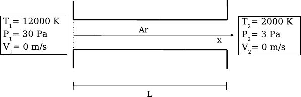
The unsteady coupling method was applied to an unsteady shock tube test case
(fig.4).
Fig. 4 Shock tube test case.
We simulated the flow field inside a 0.5 m long tube, connecting two infinitely large
tanks filled with Argon at different thermodynamic conditions. A membrane at the
interface between the first tank and the tube divides the two regions where the fluid
421
G. Abbate, B.J. Thijsse, and C.R. Kleijn
is in different conditions: in the left tank it is at a pressure P
1
= 30 Pa and at a
temperature T
1
= 12000 K, while in the right tank and in the tube it is at a pres-
sure P
2
= 3 Pa and at a temperature T
2
= 2000 K. At t = 0 the membrane breaks
and the fluid can flow from one region to the other. Two different waves will start
travelling from the left to the right with two different velocities: a shock wave and a
contact discontinuity. The shock wave produces a rapid increase of the temperature
and pressure of the gas passing through it, while through the contact discontinuity,
the flow undergoes only a temperature, and not a pressure, variation [25, 26].
The thermodynamic conditions inside the infinitely large tanks remain constant. For
this reason the two tanks can be modeled with an inlet and an outlet boundary con-
dition.
Inside the tube, we suppose that the flow is one-dimensional. Upstream (left) from
the shock, the gas has a high temperature and relatively high pressure, and gradient
length scales are small. Downstream (right) from the shock, both temperature and
pressure are much lower, and gradient length scales are large. As a result, the contin-
uum breakdown parameter Kn
max
(using local values of Q
ref
) is high upstream from
the shock, and low downstream of it. In the hybrid DSMC-CFD approach, DSMC
is therefore applied upstream, and CFD is applied downstream. The continuum grid
is composed of 100 cells in the x-direction and 1 cell in the y-direction, while the
code automatically refines the mesh in the DSMC region to fulfil its requirements.
The coupling time step is
∆
t
coupling
= 4.0×10
−6
sec. and ensemble averages of the
DSMC solution were made on 30 repeated runs.
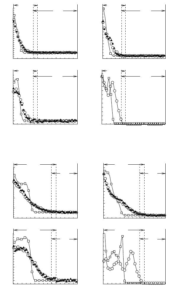
In figs. 5 and 6 the pressure (a), temperature (b), and velocity (c) inside the tube
after 1.5 ×10
−5
sec. and 3.0 ×10
−5
sec. respectively, evaluated with the coupled
DSMC-CFD method, are compared to the results of a full DSMC simulation. The
latter was feasible because of the 1-D nature of the problem. Results obtained with a
full CFD simulation are shown as well. The full DSMC solution is considered to be
the most accurate of the three. In figs. 5(d) and 6(d) also the continuum breakdown
parameter, computed using the coupled method, is compared to that same parameter
computed with the full CFD simulation.
From the results shown in figs. 5 and 6, it is clear that the full CFD approach fails
due to the high values of the local Kn number caused by the presence of the shock.
It predicts a shock thickness of ≈2 cm, which is unrealistic since even in continuum
conditions the shock thickness is one order of magnitude greater than the mean free
path (
λ
≈ 1 cm) [37]. In the full DSMC approach, therefore, the shock is smeared
over almost 10 cm. The results obtained with the hybrid approach are virtually iden-
tical to those obtained with the full DSMC solver (maximum difference < 1.5%)...,
but were obtained in less than one fifth of the CPU time.
Comparing figs. 5 and 6 it is also possible to see how the DSMC and CFD regions
adapt in time to the flow field evolution.
422
Hybrid N-S/DSMC Simulations of Gas Flows with Rarefied-Continuum Transitions
x (m)
Pressure (Pa)
0 0.1 0.2 0.3
0
5
10
15
20
25
(a)
CFD
DSMC
x (m)
Temperature (K)
0 0.1 0.2 0.3
2000
4000
6000
8000
10000
(b)
CFD
DSMC
x (m)
Velocity (m/s)
0 0.1 0.2 0.3
0
400
800
1200
(c)
CFD
DSMC
x (m)
Kn
0 0.1 0.2 0.3
0
0.2
0.4
0.6
max
(d)
CFD
DSMC
Fig. 5 Pressure (a), temperature (b), velocity (c) and continuum breakdown parameter Kn
max
(d)
in the tube after 1.5 ×10
−5
sec. CFD (), DSMC (N), Hybrid (O).
x (m)
Kn
0 0.1 0.2 0.3
0
0.2
0.4
0.6
max
(d)
DSMC
CFD
x (m)
Temperature (K)
0 0.1 0.2 0.3
2000
4000
6000
8000
10000
(b)
CFD
DSMC
x (m)
Velocity (m/s)
0 0.1 0.2 0.3
0
400
800
1200
(c)
CFD
DSMC
x (m)
Pressure (Pa)
0 0.1 0.2 0.3
0
5
10
15
20
25
(a)
CFD
DSMC
Fig. 6 Pressure (a), temperature (b), velocity (c) and continuum breakdown parameter Kn
max
(d)
in the tube after 3.0 ×10
−5
sec. CFD (), DSMC (N), Hybrid (O).
423
G. Abbate, B.J. Thijsse, and C.R. Kleijn
4.1.1 Sensitivity to numerical parameters
In this section, the sensitivity of the coupled approach to various numerical param-
eters is addressed. In particular, the influence of the size of the overlap region, the
DSMC noise, and the Courant number, based on the time interval at which DSMC
and CFD are coupled, are analysed.
Overlap region: Both DSMC and N-S equations are solved in the overlap region
(fig.3). The dependence of the results on the size of the overlap region is inves-
tigated by considering various overlap sizes:
λ
/3, 3
λ
, 6
λ
, 12
λ
, where
λ
is the
mean free path length.
time (
Shock velocity (m/s)
0 10 20 30 40
1000
1500
2000
2500
3000
3500
(a)
µ
s)
time (
Shock thickness (m)
0 10 20 30 40
0
0.04
0.08
0.12
µ
s)
(b)
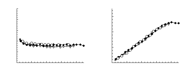
Fig. 7 Computed shock velocity (a) and shock thickness (b) as a function of time, for different
sizes of the overlap region.
λ
/3 (N), 3
λ
(∇), 6
λ
(), 12
λ
(O).
Fig.7 shows the evolution in time of respectively the shock velocity (a) and its
thickness (b), evaluated using the different overlap sizes. From this picture it is
clear that the overlap size does not strongly influence the results of the simula-
tion.
If we fix the transition between the CFD and DSMC regions at the location where
Kn = 0.05 and the overlap region is large, it is important to use an asymmetric
overlap that is bounded on one side by the location where Kn = 0.1. Otherwise,
if the overlap region would extend into regions where Kn > 0.1, the program
would solve the N-S equations in a region where the continuum hypotheses are
no longer valid. As a result, instability problems appear.
Number of repeated runs for the ensemble average: To analyze the effect of the
noise in the DSMC solution on the coupling method we considered different
numbers of repeated runs for the ensemble average: 5, 30 and 50 runs.
From a comparison (not shown) of the evolution of the shock velocity and thick-
ness similar to the one in fig.7, since the maximum differences in the solutions
were all below 5%, it became clear that also the number of repeated runs, over
424
Hybrid N-S/DSMC Simulations of Gas Flows with Rarefied-Continuum Transitions
time (
Shock velocity (m/s)
0 10 20 30 40
1000
1500
2000
2500
3000
3500
(a)
µs)
time (
Shock thickness (m)
0 10 20 30 40
0
0.04
0.08
0.12
µs)
(b)
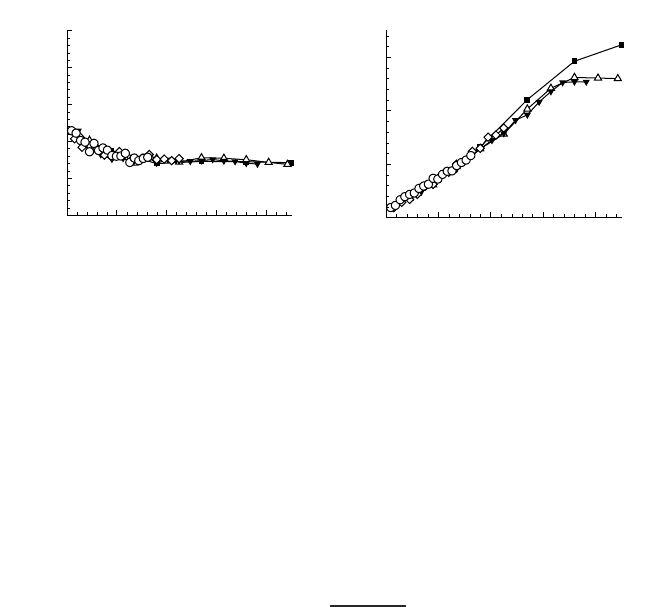
Fig. 8 Computed shock velocity (a) and shock thickness (b) for different coupling Courant num-
bers. C = 1.46 (), C = 0.73 (△), C = 0.36 (H), C = 0.24 (♦), C = 0.15 (O).
which we average, does not strongly influence the results of the method.
The limited sensitivity of our method to both the size of the overlap region and the
reduction of noise through ensemble averaging demonstrates the clear advantage
of our Dirichlet-Dirichlet coupling method as compared to Neumann-Neumann
coupling schemes [15, 16, 18, 19], which show a strong sensitivity to noise.
Courant number based on the coupling time step: In this section we study the ef-
fect of varying the coupling Courant number defined as:
C = C
r
∆
t
coupling
∆
x
CFD
, (68)
where
∆
x
CFD
is the size of CFD cells and C
r
the molecules most probable veloc-
ity.
In fig.8 we present the evolution in time of both the shock velocity (a) and its
thickness (b) for different coupling Courant numbers: 0.15, 0.24, 0.36, 0.73
and 1.46. In order to vary the Courant number we fixed
∆
x
CFD
= 0.005 m and
C
r
= 912 m/s and we considered different values of the coupling time step be-
tween 8.0 ×10
−7
sec. and 8.0 ×10
−6
sec. In terms of multiples of the mean
collision time, which is approximately
∆
t
c
= 6.0 ×10
−6
sec., this corresponds
respectively to 0.13
∆
t
c
−1.3
∆
t
c
. Only in the case where the Courant number
C = 1.46 > 1, the solution is found to deviate from the other solutions. In this
case in fact the shock thickness is higher than for the other cases and the error is
due to the appearance of instability effects (fig.9).
In order to be sure about the Courant number effects, we also varied the Courant
number by varying
∆
x
CFD
at fixed
∆
t
coupling
and fixed C
r
, and by varying C
r
at
fixed
∆
x
CFD
and
∆
t
coupling
.
In all cases, instabilities were found to arise when C > 1, as expected. It is there-
fore necessary to keep the Courant number, based on the coupling time step, the
425
G. Abbate, B.J. Thijsse, and C.R. Kleijn
x (m)
Pressure (Pa)
0 0.1 0.2 0.3 0.4 0.5
0
5
10
15
20
25
x (m)
Pressure (Pa)
0.2 0.3
2
4
6
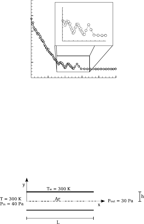
Fig. 9 Instability problems for Courant number C = 1.46.
CFD cell size and the molecules most probable velocity, smaller than 1.
4.2 Rarefied Poiseuille flow
The steady-state coupling method in two dimensions was applied to a plane Poiseuille
flow (fig.10).
Fig. 10 Rarefied Poiseuille flow.
We consider a flow of Argon at a temperature T = 300 K in a small channel of height
426