Lazinica A. (ed.) Particle Swarm Optimization

Подождите немного. Документ загружается.

Particle Swarms for Continuous, Binary, and

Discrete Search Spaces

Lisa Osadciw and Kalyan Veeramachaneni

Department of Electrical Engineering and Computer Science, Syracuse University

NY, U.S.A.

1. Introduction

Swarm Intelligence is an adaptive computing technique that gains knowledge from the

collective behavior of a decentralized system composed of simple agents interacting locally

with each other and the environment. There is no centralized command or control dictating

the behavior of these agents. The local interactions among these agents cause a global

pattern to emerge from which problems are solved. The foundation of swarming theory was

given in 1969. Two scientists, Keller and Segel, in their paper, “Slime mold aggregation”,

challenged the traditional pacemaker theory [47]. They suggested that the slime mold

aggregation is a result of mutual interactions among different cells rather than the

traditional belief that the aggregation is directed by a pacemaker cell. This theory became

the basis for swarm theory. In emergent systems, an interconnected system of rel- atively

simple agents self-organize to form a more complex, adaptive, higher-level behav- ior. To

attain this complex behavior, these elements follow simple rules (e.g., the rule defined by

the “Social Impact Theory” [18]). Examples of such systems can be found abundant in

nature including ant colonies, bird flocking, animal herding, honey bees, bac- teria, and

many more. These natural systems are optimizing using certain criteria during local

interactions so that the routes optimize as ants trace the way to food. The ants may be

designed to achieve goals other than locating food adding more dimensions to the basic

algorithm. From closely observing these highly decentralized behaviors, a “swarm-like”

algorithm emerges such as the Ant Colony Optimization (ACO) and Particle Swarm Opti-

mization (PSO). The ACO and PSO have been applied successfully to solve real-world

optimization problems in engineering and telecommunication [8, 9]. Swarm Intelligence

algorithms have many features in common with Evolutionary Algorithms. Evolutionary

algorithms are population based stochastic algorithms in which the population evolves over

a number of iterations using simple operations. Like EA, SI models are population- based.

The system is randomly initialized with a population of individuals, i.e., potential solutions.

These individuals move in search patterns over many iterations following sim- ple rules,

which mimic the social and cognitive behavior of insects or animals as they try to locate a

prize or optima. Unlike EA, SI based algorithms do not use evolutionary opera- tors such as

crossover and mutation.

Particle Swarm Optimization algorithm (PSO) was originally by Kennedy and Eber- hart in

1995 [18], and with social and cognitive behavior, has become widely used for optimization

Particle Swarm Optimization

452

problems found in engineering and computer science. PSO was inspired by insect swarms

and has since proven to be a powerful competitor to other evolutionary algorithms such as

genetic algorithms [41].

Comparisons between PSO and the standard Genetic algorithms (another kind of evo-

lutionary algorithms) have been done analytically based on performance in [41]. Com-

pared to Genetic algorithms the PSO tends to converge more quickly to the best solution.

The PSO algorithm simulates social behavior by sharing information concerning the best

solution. An attraction of some sort is formed with these “better” solutions helping improve

their own best solution until all converge to the single “best” solution. Each par- ticle

representing a single intersection of all search dimensions.

The particles evaluate their positions using a fitness that is in the form of a mathemati- cal

measure using the solution dimensions. Particles in a local neighborhood share memo- ries

of their “best” positions; then they use those memories to adjust their own velocities and,

thus, positions. The original PSO formulae developed by Kennedy and Eberhart were

modified by Shi and Eberhart [68] with the introduction of an inertia parameter,

, that

was shown empirically to improve the overall performance of PSO.

The number of successful applications of swarm optimization algorithms is increasing

exponentially. The most recent uses of these algorithms include cluster head identification in

wireless sensor networks in [69], shortest communication route in sensor networks in [9]

and identifying optimal hierarchy in decentralized sensor networks.

In the next section the particle swarm for continuous search spaces is presented. The

continuous particle swarm optimization algorithm has been a research topic for more than

decade. The affect of the parameters on the convergence of the swarm has been well stud-

ied in. The neighborhood topolgies and different variations are presented extensively in. In

this chapter we will focus on the binary and the discrete version of the algorithm. The

binary version of the algorithm is presented in section 2.2 and the discrete version of the

algorithm is presented in section 2.3. The binary and the discrete version of the algorithm-

make the particles search in the probablistic search space. The infinite range of the veloci-

ties are transformed into a bounded probabilistic space. The transformations and the

algorithms are detailed in this chapter. The affect of the parameters are briefly detailed in

this chapter. The performance of these algorithms are presented on simple functions. The

chapter is accompanied by a code written in MATLAB that can be used by the readers.

2. Particle Swarms for Continuous Spaces

The PSO formulae define each particle as a potential solution to a problem in a D-

dimensional space with the i

particle represented as

123

( , , ,....... )

iiii iD

xxx x= . Each particle

also maintains a memory of its previous best position, designated as pbest,

123

( , , ,....... )

iiii iD

Pppp p=

, and a velocity along each dimension represented as

123

( , , ,....... )

iiii iD

Vvvv v= . In each generation, the previous best, pbest, of the particle com-bines

with the best fitness in the local neighborhood, designated gbest. A velocity is com- puted

using these values along each dimension moving the particle to a new solution. The portion

of the adjustment to the velocity influenced by the individual’s previous best posi- tion is

considered as the cognition component, and the portion influenced by the best in the

neighborhood is the social component.

In early versions of the algorithm, these formulae are

Particle Swarms for Continuous, Binary, and Discrete Search Spaces

453

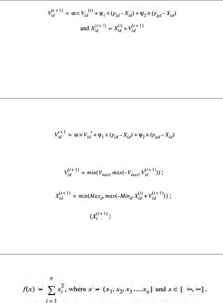
(1)

(2)

Constants

and

determine the relative influence of the social and the cognition

components, and the weights on these components are set to influence the motion to a new

solution. Often this is same value to give each component (the cognition and the social

learning rates) equal weight. A constant,

max

V , is often used to limit the velocities of the

particles and improve the resolution of the search space.

The algorithm is primarily used to search continuous search spaces. The pseudocode of the

algorithm for the continuous search spaces is shown in Figure 1.

Algorithm PSO:

For t= 1 to the max. bound of the number on generations,

For i=1 to the population size,

For d=1 to the problem dimensionality,

Apply the velocity update equation:

where P

is the best position visited so far by X

is the best position visited so far by any particle

Limit magnitude:

Update Position:

End- for-d;

Compute fitness of

;

If needed, update historical information regarding Pi and Pg;

End-for-i;

Terminate if Pg meets problem requirements;

End-for-t;

End algorithm.

Figure 1. Pseudocode for the Continuous PSO Algorithm

Example 1: Continuous PSO on a simple spheres function : Minimize the function

The MATLAB code for the above problem as solved by the particle swarm optimiza- tion

algorithm is provided along with the chapter. In the following solution 10 particles are

Particle Swarm Optimization

454

randomly intialized in the search space. The evolution of the particles after 10, 100 and 1000

iterations in the search space are shown for a 2-D problem.

3. Binary Search Spaces

The binary version of the Particle swarm optimization is needed for discrete, binary search

spaces. Many variables in the sensor management problems are binary, for example the

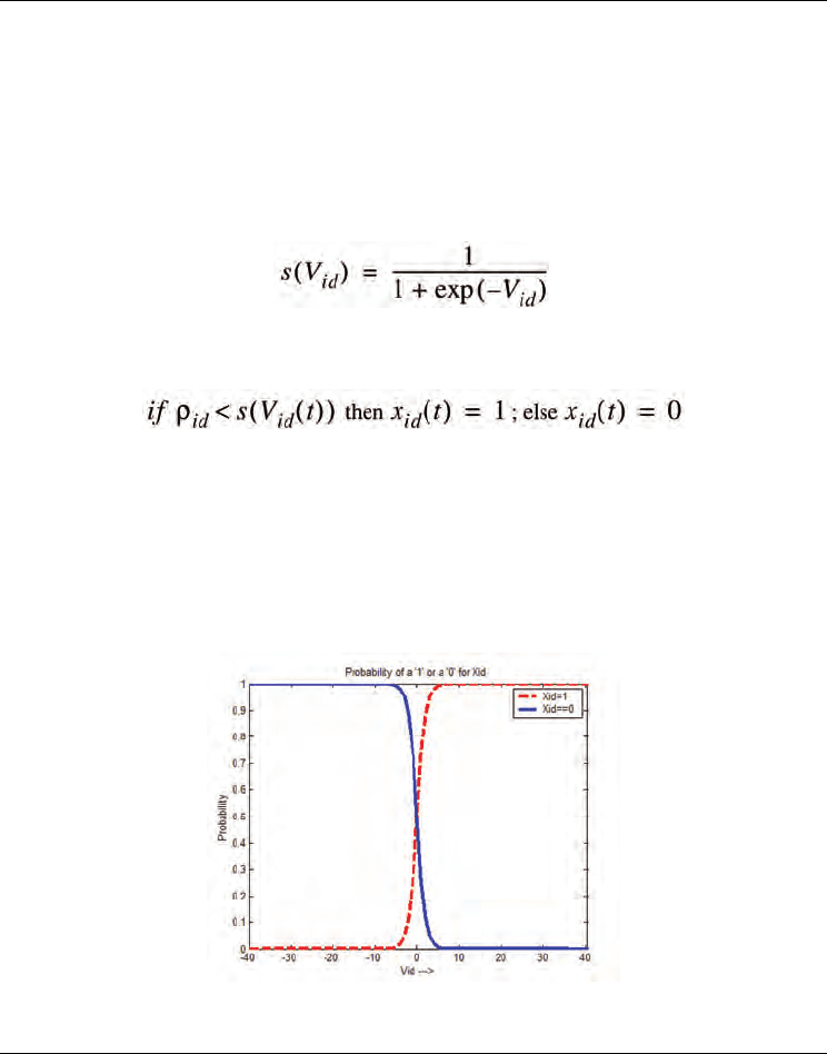
fusion rule for binary hypothesis testing is binary valued. A sigmoid function trans- forms

the infinite range of the velocities to a requisite 0 or 1. The sigmoid function is

(3)

where V

is the velocity of the ith particle along the dth dimension. The velocity update

equation remains the same as section 2.1. The position update equation is modified as

(4)

where

is a random number drawn from a uniform distribution between

0,1U

⎡⎤

⎣⎦

These formula are iterated repeatedly over each dimension of each particle, and updating

the pbest vector if a better solution is found. This is similar to the PSO for continuous search

spaces.

By following the above procedure, we transform the entire continuous velocity space,

,−∞ ∞

⎡⎤

⎣⎦

, is transformed into a one or zero for that dimension. The probability of 1

and probability of zero for different velocities is shown in Figure 2.

Figure 2. Probability of X

=1 and X

=0 given the V

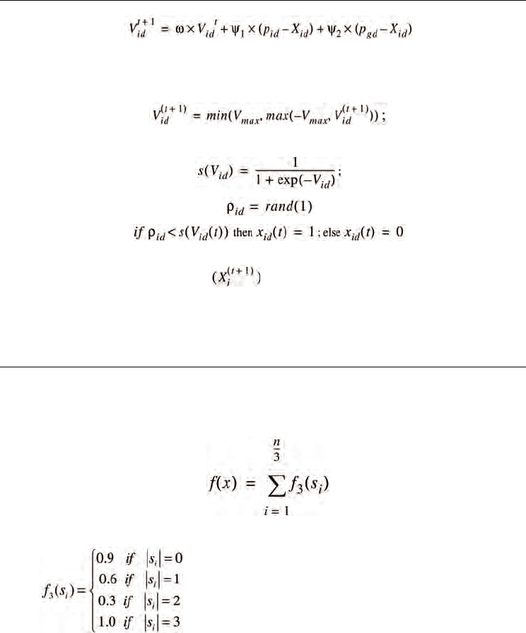
Algorithm Binary PSO:

For t= 1 to the max. bound of the number on generations,

For i=1 to the population size,

For d=1 to the problem dimensionality,

Apply the velocity update equation:

Particle Swarms for Continuous, Binary, and Discrete Search Spaces

455

where P

is the best position visited so far by X

is the best position visited so far by any particle

Limit magnitude:

Update Position:

End- for-d;

Compute fitness of ;

If needed, update historical information regarding Pi and Pg;

End-for-i;

Terminate if Pg meets problem requirements;

End-for-t;

End algorithm.

Figure 3. Pseudocode for the Binary PSO Algorithm

Example 2: Goldberg’s Order-Three Problem

Groups of three bits are combined to form disjoint subsets and the fitness is evaluated using

where each si is a disjoint 3-bit substring of x and

where |si| denotes the sum of the bits in the 3-bit substring

2. 3 Particle Swarms for Discrete Multi Valued Search Spaces

Extending this binary model of PSO, a discrete multi-valued particle swarm for any range of

discrete values is described in detail. Many real world optimization problems, including

signal design, power management in sensor networks, and scheduling have vari- ables

which have discrete multi-values. This need is increasing as more problems are being solved

by particle swarm optimization based algorithm [73, 74]. It can be argued instead that

Particle Swarm Optimization

456

discrete variables can be transformed into an equivalent binary representation, and the

binary PSO can simply be used. However, the range of the discrete variables does not

typically correspond to a power of 2 for the equivalent binary representation. This then

generates a range of values exceeding the real range resulting in an unbalanced conver-

gence and more iterations than necessary. For example, a discrete variable ranging from 0

to5 [0,1,2,3,4,5] requires a minimum of three bit binary representation, which ranges

between [0-7]. Special conditions need to be added reducing the algorithms efficiency to

manage the values beyond the original maximum, which in this example is, 6 & 7. Another

important factor is that the Hamming distances between the two discrete values, undergoes

a non-linear transformation using the equivalent binary representation. This often adds to

the complexity to the search process. The inefficiency emerges as an increase in the

dimensions of the particle adding more variables to the search. For these reasons, a discrete

multi valued PSO is more efficient and should be used for discrete ranges greater than 2.

Previously, researchers simply enhanced the performance of the binary PSO to fix the

efficiency. Al-Kazemi, et al. [75], improved the original binary PSO algorithm by modify-

ing the way particles interact. The research on designing a PSO for discrete multi-valued

problems, however, has been sparse. In MVPSO [74], Jim, et al, extended the binary PSO by

creating a multi dimensional particle. Each dimension of the original problem is subdi-

vided into three dimensions for a ternary problem. Each dimension of the particle is a real

valued number and is transformed into a number in the range of [0 1] using the sigmoid

function. After a series of transformations, the three numbers ultimately represent the

probability of having a one of three discrete values for a ternary system. The extra trans-

formations bring us closer to the new discrete multi-valued PSO except many operations are

added. The transition of a particle or position update is probabilistic similar to the binary

PSO.

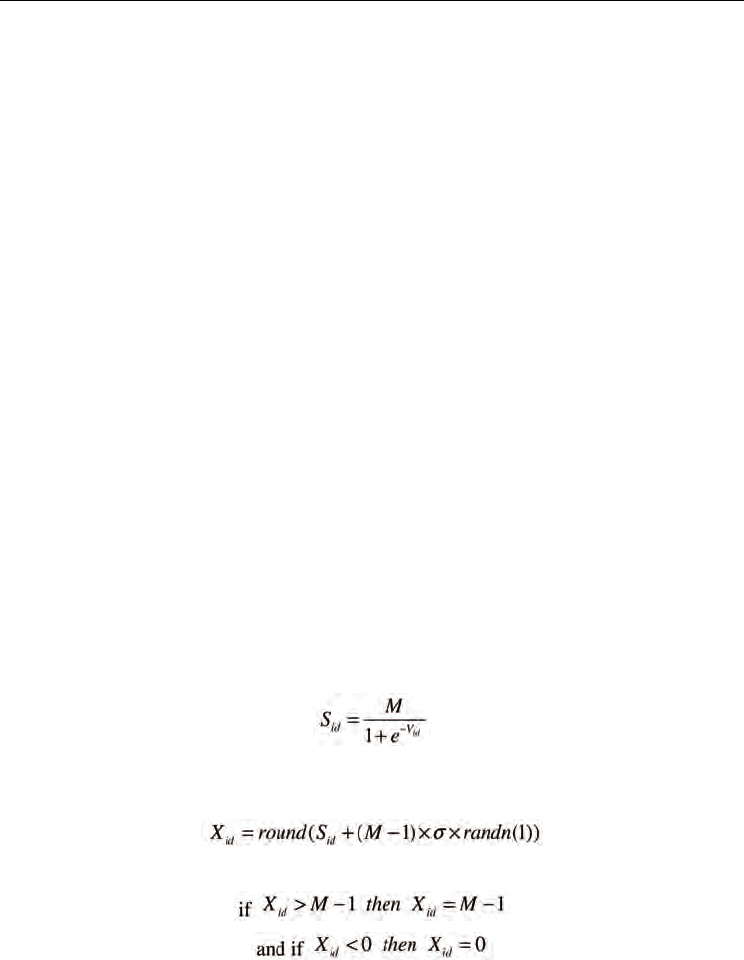
For discrete multi valued optimization problems, the range of variables lie between 0 and

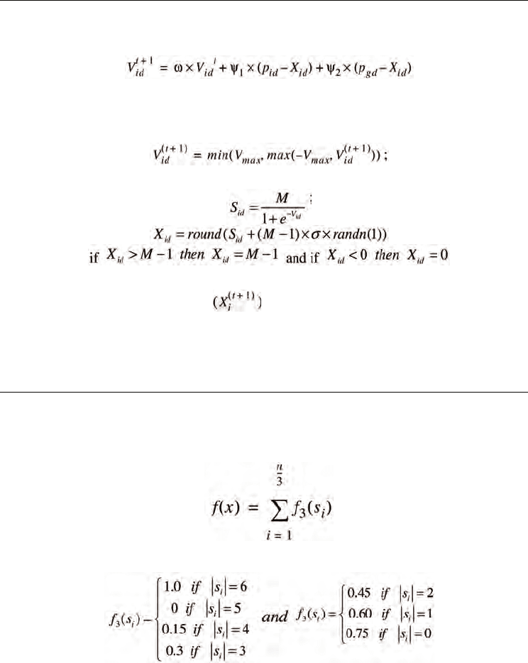
M-1, where ‘M’ implies an M-ary number system. The same velocity update and par- ticle

representation are used in this algorithm. The position update equation is, however, change

as follows.

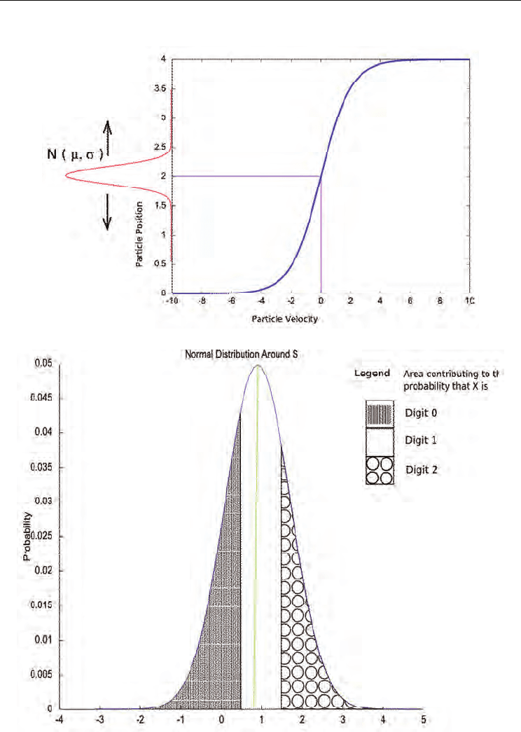
1. Transform the velocity using

(5)

2. A number is the generated using a normal distribution with

and

parameters.

(6)

3. The number is rounded to the closest discrete variable with the end points fixed.

(7)

(8)

4. . The velocity update equation remains the same as (1). The positions of the particles are

discrete values between 0 and M-1. Now for any given S

, we have an associated

probability for any number between [0, M-1]. However, the probability of drawing a

num- ber randomly reduces based on its distance from S

according to the Figure 4. In

Particle Swarms for Continuous, Binary, and Discrete Search Spaces

457

the subsection, the relation between Sid and the probability of a discrete variables is

given.

Figure 4. Transformation of the Particle Velocity to a Discrete Variable

Figure 5. Probabilities of Different Digits Given a Particular S

Particle Swarm Optimization

458

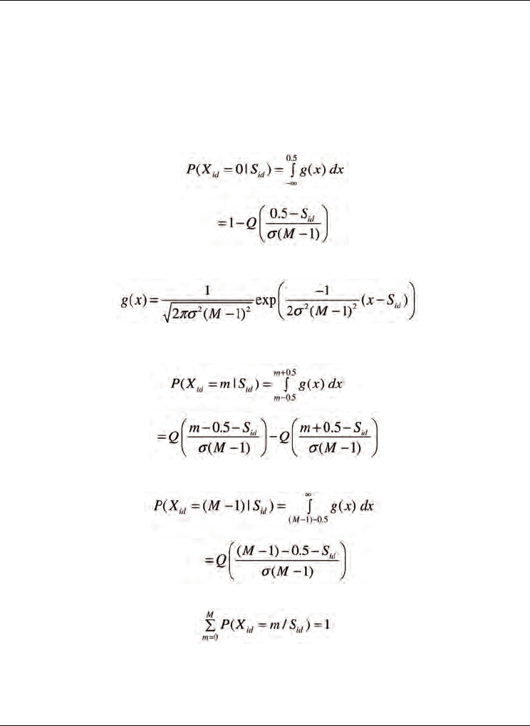
Probability of a discrete value ‘m’: For a given S, a number is generated using a normal

distribution with the mean as S and standard deviation

for an M-ary system. Based on

this normal distribution and equation (7), the probability for a specific discrete variables

given S can be calculated based on the area under that region of the Gaussian curve. For

example for a ternary system, given an S = 0.9 and

= 0.8, the areas of the Gaussian curve

that will contribute to different digits are shown in Figure 5. For a S

, the probability of a

discrete variable having a value ‘m’ is given by:

m=0,

(9)

where Q is the error function. The function g(x) is

(10)

with m in the range 1 to M-2, the conditional probability of achieving X

given a previous

value is

(11)

For m = M-1, the conditional probability is

(12)

Note that

(13)

One can significantly control the performance of the algorithm using these equations. For

example, controlling the

controls the standard deviation of the Gaussian and, hence, the

probabilities of various discrete variables.

Algorithm Discrete PSO:

For t= 1 to the max. bound of the number on generations,

For i=1 to the population size,

Particle Swarms for Continuous, Binary, and Discrete Search Spaces

459

For d=1 to the problem dimensionality,

Apply the velocity update equation:

where P

is the best position visited so far by X

is the best position visited so far by any particle

Limit magnitude:

Update Position:

End- for-d;

Compute fitness of

;

If needed, update historical information regarding Pi and Pg;

End-for-i;

Terminate if Pg meets problem requirements;

End-for-t;

End algorithm.

Figure 6. Psuedo Code for Particle Swarms for Discrete Multi Valued Search Spaces

Example 3: Sastry-Veermachaneni-Osadciw Function for Ternary Systems

Groups of three digits are combined to form disjoint subsets and the fitness is evalu- ated using

where each s

is a disjoint 3-bit substring of x and

where |s

| denotes the sum of the digits in the 3-digit substring.

2.4 Particle Swarms for Mixed Search Spaces

Mixed search spaces imply that the solution to the problem is composed of binary, dis- crete

and continuous variables. The solution can be any combination of two. The particle swarm

Particle Swarm Optimization

460

optimization algorithms operators work independently on each dimension making it

possible for mixing different variable types into one single particle. In Genetic algo- rithms,

however, the crossover operator needs to be designed independently for the differ- ent

variable types. The swarm algorithm will call upon the different position update formulae

based on the type of the variable. The pseudo code is given in the following fig ure.

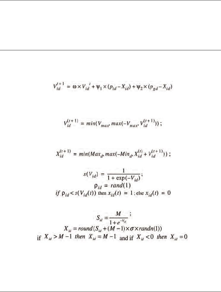
Algorithm PSO for Mixed Search Spaces:

For t= 1 to the max. bound of the number on generations,

For i=1 to the population size,

For d=1 to the problem dimensionality,

Apply the velocity update equation:

where P

is the best position visited so far by X

is the best position visited so far by any particle

Limit magnitude:

Update Position:

if X

is continuous valued

else if X

is binary valued

elseif X

is discrete valued

End- for-d;

Compute fitness of (X



+ 1

);

If needed, update historical information regarding Pi and Pg;

End-for-i;

Terminate if Pg meets problem requirements;

End-for-t;

End algorithm.

Figure 7. Pseudo code for mixed search spaces