Massoud M. Engineering Thermofluids: Thermodynamics, Fluid Mechanics, and Heat Transfer

Подождите немного. Документ загружается.

622 Va. Two-Phase Flow and Heat Transfer: Two-Phase Flow Fundamentals

Constants C

, C

, and C

may be obtained from the Martinelli-Nelson or the Thom

correlation. Figure Va.2.3 gives the values of constants C

, C

, and C

according

to Thom’s correlation.

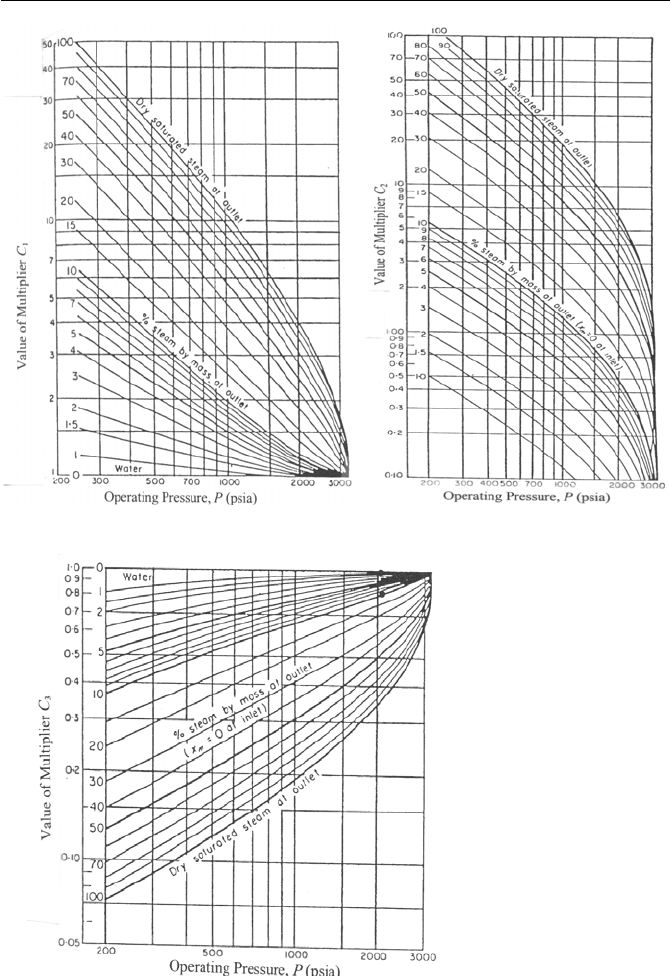
Example Va.2.9. Solve Example Va.2.8 based on the Separated Flow Model.

Solution: The same total pressure drop is applicable in the preheating section for

both HEM and SFM. For the boiling section, we use Figure Va.2.3 for (∆P)

fric

(∆P)

acc

and (∆P)

grav

respectively. These result in: C

≈ 8.5, C

≈ 14, and C

≈ 0.24.

Substituting the constants in Equation Va.2.30, we find:

)(

sptpfric

=∆ =

=×

××

5.8

00135.03)3.318(

02.0

0199.0

1.74 kPa

)](/[)(

CGP

ftpacc

=∆ = (318.3)

× 0.00135 × 7.8 = 1.90 kPa

)(cos)(

CgLP

fbtpgrav

βρ

=∆ = 9.81 × (3/0.00135) × 0.24 = 5.2 kPa

Therefore, total pressure drop over the tube is found as:

∆P

total

= (0.068 + 1.74) + (0.018 + 1.90) + (7.8 + 5.2) = 16.7 kPa

This result is in reasonable agreement with the result obtained from the homoge-

nous model in Example Va.2.8.

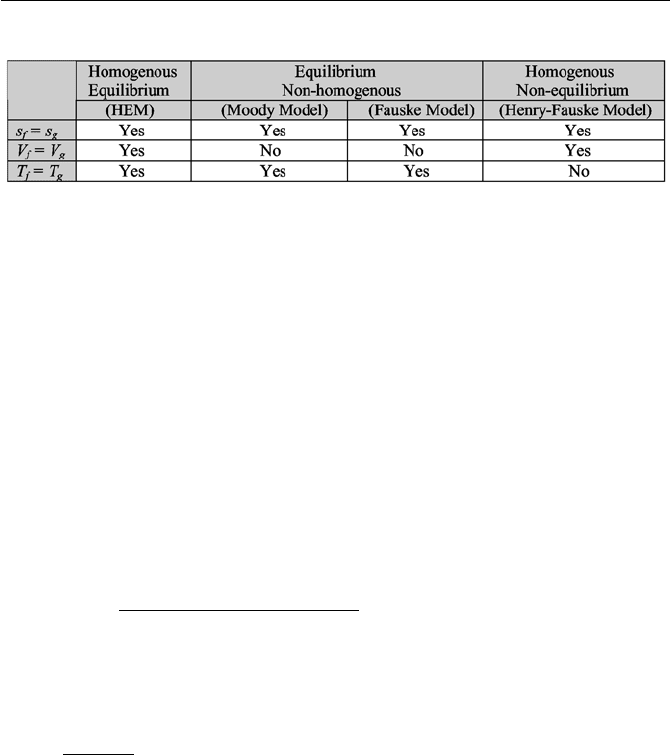
3. Two Phase Critical Flow

Similar to the critical flow of compressible, single-phase fluid, as discussed in

Chapter IIIc, flow of a two-phase mixture in a channel may also become critical.

For cases where saturated water is contained under pressure, opening of a valve or

sudden burst of a connecting pipe results in expulsion of the tank inventory. In

such a case, the saturated water may partially flash to steam as it approaches the

break area, which is at much lower pressure. We will seek an analytical solution

for the two-phase critical flow of water and steam under the following conditions;

flow is homogeneous (V

= V

), thermodynamic equilibrium exists between the

phases (T

= T

), and the process is isentropic. These assumptions lead to the de-

termination of critical flow for HEM. Maintaining the assumption of an isentropic

process, analytical solutions are also extended to two equilibrium non-homo-

genous cases. The first case uses a slip ratio calculated from either the Moody or

the Fauske model. The second case uses models from Burnell and Henry-Fauske.

These cases are summarized in Table Va.3.1 and then discussed in detail next.

3. Two Phase Critical Flow 623

Figure Va.2.3. Coefficients for frictional, acceleration, and gravitational pressure drop

(Thom 1964)

624 Va. Two-Phase Flow and Heat Transfer: Two-Phase Flow Fundamentals

Table Va.3.1. Various critical flow models

3.1. Two-Phase Critical Flow (Homogeneous Equilibrium Flow)

This model is based on solving the conservation equations of mass and energy, in

conjunction with the equations of state, under steady-state condition. The conser-

vation equation of mass becomes:

VAm



= constant IIa.5.2

where

is the mixture density. Note that no distinction is made between V

and

. The energy equation for the mixture, using the upstream stagnation condition

(shown with subscript o), becomes:

= h + V

/2 IIIc.2.1

We may substitute for velocity from Equation IIIc.2.1 into IIa.5.2 and write the re-

sult in terms of mass flux:

()

[]

gfo

xhhxh

vv)1(

)1(2

2/1

+−

−−−

Va.3.1

where we also made use of the equation of state for h = (1 – x)h

+ xh

. If we sub-

stitute for quality calculated from the mixture entropy

−

into Equation Va.3.1, we obtain a relation that is solely a function of pressure. By

iteration with the steam tables, we can then find a pressure that maximizes mass

flux. Alternatively, we may express all thermodynamic properties and their de-

rivatives as functions of pressure (examples of such functions are given in Appen-

dix II, Table A.II.3). To find the pressure that maximizes mass flux, we then sub-

stitute these functions into Equation Va.3.1, take the derivative of G and set it

equal to zero.

3.2. Two-Phase Critical Flow (Equilibrium Non-homogeneous Flow)

This is similar to the homogenous flow, but we must account for V

≠ V

. The

mass balance becomes:

3. Two Phase Critical Flow 625

−

===

ααα

Va.3.2

The energy equation can be partitioned to account for the contribution of each

phase as follows:

()

+−=

hxh

Va.3.3

To find G, we first substitute for void fraction from Equation Va.1.3. We then

find V

and V

in terms of G from Equation Va.3.1, substitute them into Equation

Va.3.2, and solve for G to obtain:

()

−−−=

fef

sshhG

Va.3.4

where in Equation Va.3.4,

* is given by:

[]

−

+−= x

xxS

vv)1(

Va.3.5

Note that in Equation Va.3.5 the slip ratio S as given by Equation Va.1.1 should

not be confused with s, the specific entropy. We now need to determine the slip

ratio such that the mass flux is maximized. There are two models for this, as dis-

cussed next.

The Moody Model. In this model, the mass flux given by Equation Va.3.4 is

maximized by setting the derivative of the kinetic energy with respect to slip ratio

equal to zero,

∂K.E./∂S = 0:

()

−

∂

xVVx

Taking the derivative and setting it equal to zero, we obtain:

Moody

= (v

)

1/3

The Moody model compares well with data in the range of 14.7 – 400 psia.

The Fauske Model. In this model, the mass flux given by Equation Va.3.4 is

maximized by setting the derivative of the flow momentum, with respect to slip

ratio, equal to zero:

626 Va. Two-Phase Flow and Heat Transfer: Two-Phase Flow Fundamentals

()

[]

01 =+−

∂

xVVx

This maximizes the axial pressure gradient for a given flow rate and steam quality.

Substituting from Equation Va.3.1 for V

and V

, introducing Equation Va.1.3 for

void fraction, and applying the chain rule for differentiation results in:

Fauske

= (v

)

1/2

Example Va.3.1. Derive the critical condition for annular flow using the conser-

vation equation for mass and momentum.

Solution: We use the thermodynamic equilibrium and non-homogenous assump-

tion, V

≠ V

. The combined continuity and momentum equations result in.

0)( =++ AdPVmVmd

ggff



Substituting from Equation V.3.2 for V

and V

in terms of G, we find:

()

0vv

−

+ G

ddP

αα

Solving for G, we obtain:

()

ddPG v/−= Va.3.6

where specific volume in Equation Va.3.6 is given by:

()

αα

−

Va.3.7

Having found the slip ratio by the Moody or the Fauske method, we express the

thermodynamic properties and their derivatives in terms of pressure and substitute

into Equation IIIa.3.6-2. For example, for the Fauske model, we use Equa-

tions IIIa.3.6-2, Va.1.3 (with

S v/v= ), and Va.3.6 to obtain (Nahavandi):

()

[]

()

[]

xxSSxSSxS

xxSx



−+++−−++−=

−

v221v222

Va.3.8

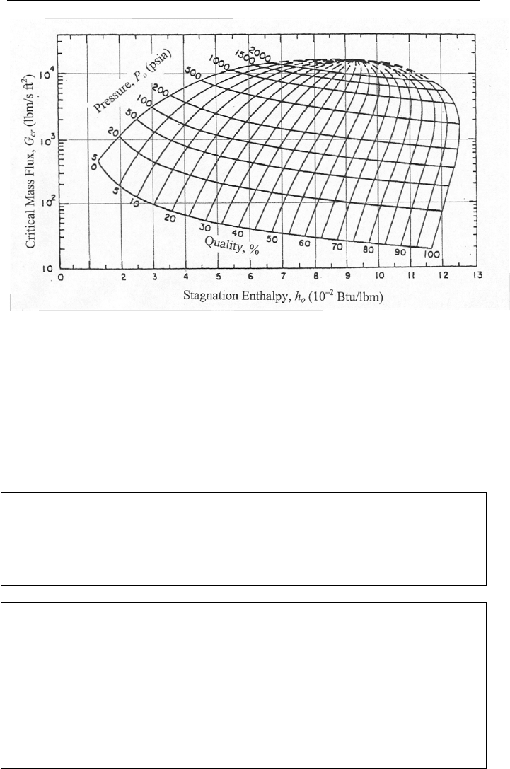
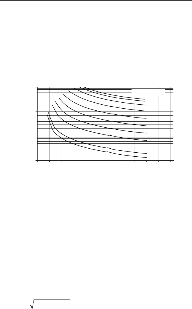
Nahavandi then plotted Equation Va.3.8 for mass flux as a function of the stagna-

tion enthalpy and pressure, as shown in Figure Va.3.1.

3. Two Phase Critical Flow 627

Figure Va.3.1. Critical mass flux versus stagnation enthalpy and pressure (Fauske)

Two observations can be made from Figure Va.3.1. First, the higher the source

stagnation pressure, the higher the mass flux at the same steam quality. Second,

for a given pressure, the critical mass flux increases with decreasing quality.

Hence, as expected, the higher the liquid content, the higher the critical mass flux.

For example, a stagnation pressure of 200 psia and x = 75% corresponds to the

same mass flux of 1000 lbm/s

⋅ft

as a stagnation pressure of only 50 psia but

steam quality of x = 11%.

Example Va.3.2. Calculate the maximum mass flux for the flow of saturated wa-

ter and steam at 2000 psia and enthalpy of 800 Btu/lbm, according to the Fauske

model.

Solution: From Figure Va.3.1 for P

= 2000 psia and h

= 800 Btu/lbm, we find

max

≈ 11,000 lbm/s⋅ft

Example Va.3.3. A discharge line is connected to a pressurized tank, which con-

tains saturated water at 1000 psia. The discharge line is equipped with a safety

valve, having a flow area of 1.4 in

. We now open the valve. Find the maximum

flow rate that leaves the tank. Assume C

= 1.

Solution: Since the discharge valve opens to atmosphere, the flow is definitely

choked. The maximum flow rate occurs at the moment that pressure is still at

1000 psia and just begins to drop. Thus from Figure Va.3.1 we find the mass flux

as G

= 10,100 lbm/s⋅ft

and the mass flow rate as:



0.8(1.4/144) × 10,100 = 78.5 lbm/s

628 Va. Two-Phase Flow and Heat Transfer: Two-Phase Flow Fundamentals

As for the Moody model, if we substitute S = (v

)

1/3

into Equation Va.3.5 and

then use the result in Equation Va.3.4, we find the following relation for the criti-

cal mass flux:

[

]

[]

3/22

)v/v)(1(v

)1(2

fgo

hxxhh

−+

−−−

Va.3.9

Similar to the Fauske mode, mass flux from the Moody model is maximized and

plotted for various values of the source stagnation pressure and enthalpy, as shown

in Figure Va.3.2.

1.E+01

1.E+02

1.E+03

1.E+04

0 200 400 600 800 1000 1200 1400 1600 1800 2000 2200

Stagnation Enthalpy, h

(Btu/lbm)

Critical Mass Flux, G

(lbm/s ft

)

14.7

400

800

1400

2000

2400

100

200

Pressure,

(psia)

Figure Va.3.2. Critical mass flux versus stagnation enthalpy and pressure (Moody)

3.3. Two-Phase Critical Flow (Homogeneous Non-equilibrium Flow)

Earlier we showed that the existence of analytical solutions was primarily due to

the isentropic process assumption. This assumption implies that the length and di-

ameter of the flow path should be such that the frictional effects are minimized.

Thermodynamic equilibrium in turn requires a reasonably long flow path to allow

the phases to reach equilibrium. As such, the shorter the flow path, the higher the

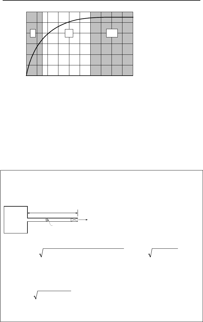
flow rate since less liquid would flash to steam. Fauske has identified three ranges

for the L/D; 0–3, 3–12, and 12–40 (Figure Va.3.3). For 0 < L/D < 3, the flow path

is too short for the phases to reach equilibrium while for 12 < L/D < 40, the flow

path allows the phases to reach equilibrium. Therefore, for the L/D range of 0 – 3,

the critical flow can be estimated from such equations as IIIa.3.46, IIIb.3.14,

IIIb.4.3, and IIIb.4.4:

()

crof

PPG −=

261.0 Va.3.10

3. Two Phase Critical Flow 629

0.1

0.2

0.3

0.4

0.5

0.6

0.0

02468

12 14

18 20

I II III

Flow Path L/D

Critical Pressure Ratio,

Figure Va.3.3. Critical pressure ratio versus flow path length over diameter (Fauske)

where in Equation Va.3.10, a discharge coefficient of 0.61 is accounted for. In

this equation, P

stands for the critical pressure. According to Fauske, the value

of P

depends on the value of the L/D ratio as shown in Figure Va.3.2. Note that,

for an orifice, (L/D = 0), P

is the actual back pressure.

In conclusion, Region I in Figure Va.3.3 is applicable to non-equilibrium flow

regimes and Region III of this figure is well suited for the HEM, since the suffi-

cient flow path length allows the phases to reach thermal equilibrium. Note that

Figure Va.3.1 would under-predict flow in Regions I and II of Figure Va.3.3.

Example Va.3.4. A pressurized tank containing saturated liquid at 2000 psia is

connected to atmosphere by a 0.5 in diameter pipe. A frictionless valve on the

pipe is suddenly opened. Find the maximum mass flux for three different pipe

lengths of L

= 0.1 ft, L

= 0.25 ft, and L

= 1 ft at this pressure.

Solution:

Find

() ()

crcr

PPPPG −=−×××=

78.36614498.382.32261.0

Next, we need to find P

– P

, having L/D. Since D = 0.5/12 = 0.042 ft

/D = 0.1/0.042 = 2.4, L

/D = 6, and L

/D = 24.

We now use Figure Va.3.3:

For L

/D = 2.4, we find P

= 0.30. Thus,

()

720,13600200078.366 =−=G lbm/s·ft

This is in good agreement with G from Figure Va.3.1 at

= 600 psia and h

= h

(2000) = 672 Btu/lbm.

For L

/D = 6.0, we find P

= 0.48. Thus,

630 Va. Two-Phase Flow and Heat Transfer: Two-Phase Flow Fundamentals

()

830,11960200078.366 =−=G

lbm/s·ft

For L

/D = 24, we find P

= 0.55.

Thus,

()

000,111100200078.366 =−=G

lbm/s·ft

As expected, G

is over-predicted compared to G

≈ 8500 lbm/s·ft

read from

Figure Va.3.1 at P

= 1100 psia and h

= h

(2000 psia) = 672 Btu/lbm.

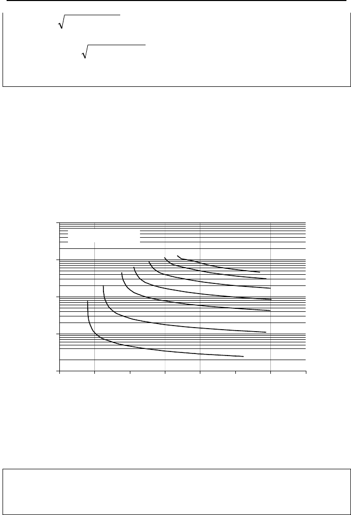
Henry (1970) and later Henry-Fauske (1971) analytically derived the relation

for two-phase critical mass flux for homogenous non-equilibrium flow, based on

the isentropic assumption. This is a reasonable assumption for short flow paths

for which the frictional pressure drop due to the wall shear forces is negligible

compared to the momentum and pressure gradient terms. The RELAP4 (Moore)

and GOTHIC (George) computer codes have tabulated the Henry correlation for

various stagnation pressure and enthalpy. These are plotted in Figure Va.3.4.

1.E+01

1.E+02

1.E+03

1.E+04

1.E+05

0 200 400 600 800 1000 1200 1400

Stagnation Enthalpy, h

(Btu/lbm)

Critical Mass Flux,

(lbm/s ft

)

200

400

800

1400

2000

Pressure, P

(psia)

Figure Va.3.4. Critical mass flux versus stagnation enthalpy and pressure (Henry non-

equilibrium model)

Example Va.3.5. In Example Va.3.5, find the maximum mass flux for L

= 0.1 ft.

Solution: From Figure Va.3.4 for P

= 2000 psia and saturated water, we find

max

≈ 10,500 lbm/s ft

3. Two Phase Critical Flow 631

3.4. Two-Phase Critical Flow

(Homogeneous Non-equilibrium, Subcooled Fluid)

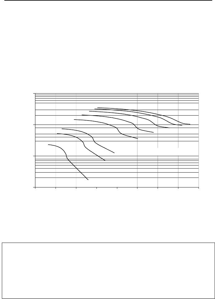
So far we dealt with saturated water and two-phase mixture. If the pressurized

water is subcooled, then the percentage of flashing decreases, resulting in higher

mass flow rate. Indeed test data indicates that the higher the degree of subcooling,

the higher the critical mass flow rate. The Henry-Fauske correlation is extended

to cover subcooled liquid. The extended Henry-Fauske correlation for maximum

mass flux is plotted as a function of stagnation enthalpy and pressure in Fig-

ure Va.3.5.

1.E+02

1.E+03

1.E+04

1.E+05

0 100 200 300 400 500 600 700 800

Stagnation Enthalpy, h

(Btu/lbm)

Critical Mass Flux,

(lbm/s ft

)

100

400

800

1400

2000

2400

Pressure,

(psia)

Figure Va.3.5. Critical mass flux versus stagnation enthalpy and pressure (Henry-Fauske

model)

Example Va.3.6. A pressurized tank containing subcooled liquid at 2000 psia is

connected to atmosphere by a frictionless valve. Find the maximum mass flux for

two cases of h

= 400 Btu/lbm and h

= 600 Btu/lbm.

Solution: We expect to obtain higher mass flux at lower upstream enthalpy. Ac-

cording to Figure Va.3.5, at a upstream pressure of 2000 psia and enthalpy of 400,

the critical mass flux is about 12,000 lbm/s. At the same pressure but enthalpy of

600 Btu/lbm, the critical mass flux is about 10,800 lbm/s.