Mayr E.W., Pr?mel H.J., Steger A. (eds.) Lectures on Proof Verification and Approximation Algorithms
Подождите немного. Документ загружается.

266 Chapter 11. Semidefinite Programming
Note that there are several other approaches for the approximation of MAXCUT
and MAXSAT. For example, in Chapter 12, the "smooth integer programming"
technique is described, which can be used if the instances are dense. For addi-
tional references on semidefinite programming and combinatorial optimization,
we refer to [Ali95, VB96, Goe97].
Our survey will be organized as follows: First, we describe the mathematical
tools necessary to understand the method of semidefinite programming (Sec-
tions 11.2-11.4). Since algorithms for solving semidefinite programs are rather
involved, we only give a sketch of the so-called interior-point method. We de-
scribe a "classical" approximation of MAXCUT, which is not based on semidefi-
nite programming (Section 11.5.1). We then show how Goemans and Williamson
applied semidefinite programming to obtain better approximation algorithms
for MAXCUT (Section 11.5.2) and analyze the quality of their algorithm. In Sec-
tion 11.6 we describe the modeling of the asymmetric problems MAXDICUT and
MAXE2SAT. A method for modeling long clauses in a semidefinite program is
described in Section 11.7.1. We review some classical approaches for MAXSAT
and explain how different MAXSAT algorithms can be combined in order to im-
prove the approximation ratio (Section 11.7.2). Section 11.8 describes the effect
of additional constraints and of a nonuniform rounding technique.
We give a formal definition of the problems considered in this chapter.
MAXCUT
Instance:
Given an undirected graph G = (V, E).
Problem: Find a partition V -- 1/1 U 112 such that the number of edges between
I11 and 112 is maximized.
We will assume that V = {1,... ,n}.
MAxDICuT
Instance:
Given a directed graph G = (V, E).
Problem:
Find a subset S C_ V such that the number of edges (i,j) E E with
tail i in S and head j in S is maximal.
MAXSAT
Instance:
Problem:
MAXkSAT,
Instance:
Problem:
Given a Boolean formula ~ in conjunctive normal form.
Find a variable assignment which satisfies the maximal number of
clauses in ~.
kEN
Given a Boolean formula ~ in conjunctive normal form with at most k
literals in each clause.
Find a variable assignment which satisfies the maximal number of
clauses in ~b.
11.2. Basics from Matrix Theory 267
MAxEkSAT, k E N
Instance: Given a Boolean formula r in conjunctive normal form with exactly k
literals in each clause.
Problem: Find a variable assignment which satisfies the maximal number of
clauses in ~.
The variables of the Boolean formula are denoted by xl,..., xn, the clauses are
C1,..., Cm. Note that each algorithm for MAXkSAT is also an algorithm for
MAxEkSAT. An important special case is k = 2.
Sometimes, weighted versions of these problems are considered.
WEIGHTED MAXCUT
Instance: Given an undirected graph G = (V, E) and positive edge weights.
Problem: Find a partition V = 111 t2 V2 such that the sum of the weights of
edges between V1 and 112 is maximized.
WEIGHTED MAXDICUT
Instance: Given a directed graph G = (V, E) and nonnegative edge weights.
Problem: Find a subset S C_ V such that the total weight of the edges (i,j) E E
with tail i in S and head j in S is maximal.
WEIGHTED MAXSAT
Instance: Given a Boolean formula r = C1 A ... A Cm in conjunctive normal
form and nonnegative clause weights.
Problem: Find a variable assignment for ~ which maximizes the total weight
of the satisfied clauses.
All results mentioned in this chapter hold for the unweighted and for the weighted
version of the problem. The approximation ratio for the weighted version is the
same as for the corresponding unweighted version. Since the modification of the
arguments is straightforward, we restrict ourselves to the unweighted problems.
11.2 Basics from Matrix Theory
In this section, we will recall a few definitions and basic properties from Ma-
trix Theory. The reader interested in more details and proofs may consult, e.g.,
[GvL86]. Throughout this chapter, we assume that the entries of a matrix are
real numbers.
An n x m matrix is called square iff n = m. A matrix A such that A = A T
is called symmetric. A matrix A such that ATA is a diagonal matrix is called
orthogonal. It is orthonormal if in addition ATA = Id, i.e., A T -- A -1.
268 Chapter 11. Semidefinite Programming
Definition 11.1.
An
eigenvector
of a matrix A is a vector x ~ 0 such that there
exists a )~ E C with A 9 x = )~ 9 x. The corresponding )~ is called an
eigenvalue.
The
trace
of a matrix is the sum of the diagonal elements of the matrix.
It is known that the trace is equal to the sum of the eigenvalues of A and the
determinant is equal to the product of the eigenvalues.
Note that zero is an eigenvalue of a matrix if and only if the matrix does not
have full rank.
Another characterization of eigenvalues is as follows:
Lemma 11.2.
The eigenvalues of matrix A are the roots of the polynomial
det(A
- )~. Id), where )~ is the free variable and Id is the identity matrix.
It is known that if A is a symmetric matrix, then it possesses n real eigenvalues
(which are not necessarily distinct). For such an n x n- matrix, the canonical
numbering of its n eigenvalues is A1 /> A2/> .../> An. The number of times that
a value appears as an eigenvalue is also called its
multiplicity.
Definition 11.3.
The
inner product
of two matrices is defined by
A.B:=
Z AIs " Bi,J = trace(A T . B).
i,j
Theorem 11.4 (Rayleigh-Ritz).
I] A is a symmetric matrix, then
AI(A) = max
xT.A.x and
An(A) = min
xT.A.x.
I1~11=1 I1~11=1
Semidefiniteness
Having recalled some of the basic matrix notions and lemmata, let us now turn
to the definitions of definiteness.
Definition 11.5. A square matrix A is
called
positive semidefinite
i] x T . A . x >/0 ) for all x E R n
\
(0}
positive definite
if x T 9 A . x > 0
In this chapter, we will abbreviate "positive semidefinite" also by "PSD."
As a corollary of Theorem 11.4, we obtain that a symmetric matrix is PSD if
and only if its smallest eigenvalue An/> 0.
11.2. Basics from Matrix Theory 269
Examples of PSD matrices. It should be noted that it is not sufficient for a
matrix to contain only positive entries to make it PSD. Consider the following
two matrices
( ) ( 1 -1)
1 4 B :=
A:-- 4 1 -1 4 "
The matrix A is not PSD. This can be seen by observing that (1,-1) 9 A-
(1,-1) T = -6. The eigenvalues of A are 5 and -3. On the other hand, the
symmetric matrix B with negative entries is PSD. The eigenvalues of B are
approximately 4.30 and 0.697.
For a diagonal matrix, the eigenvalues are equal to the entries on the diagonal.
Thus, a diagonal matrix is PSD if and only if all of its entries are nonnegative.
Also by the definition, it follows that whenever B and C are matrices, then the
matrix
is PSD if and only if B and C are PSD. This means that requiring some matrices
A1,..., Ar to be PSD, is equivalent to requiring
one
particular matrix to be PSD.
Also, the following property holds: If A is PSD, then the k • k-submatrix obtained
from A by eliminating rows and columns k + 1 to n is also PSD.
As a final example, consider the symmetric matrix
(1 a)
a 1 ... a
iiilix
with ones on the diagonal and an a everywhere else. A simple calculation reveals
that its eigenvalues are 1 + a 9 (n - 1) (with multiplicity 1) and 1 - a (with
multiplicity n - 1). Hence, the matrix is PSD for all
-1/(n -
1) ~< a ~< 1.
Further properties.
In most places in this chapter, we will only be concerned
with matrices A which are symmetric. For symmetric matrices, we have the
following lemma:
Lemma 11.6.
Let A be an n • n symmetric matrix. The following are equiva-
lent:
- A is PSD.
- All eigenvalues of A are nonnegative.
- There is an n • n-matrix B such that A = B T 9 B.
270 Chapter 11. Semidefinite Programming
Note that given a symmetric PSD matrix A, the decomposition A =
B T 9 B
is
not unique, since the scalar product of vectors is invariant under rotation, so
any rotation of (the vectors given by) matrix B yields another decomposition.
As a consequence, we can always choose B to be an upper triangular matrix in
the decomposition.
Goemans-Williamson's approximation algorithm uses a subroutine which com-
putes the "(incomplete) Cholesky decomposition" of a given PSD symmetric
matrix A. The output of the subroutine is a matrix B such that A =
B T 9 B.
This decomposition can be performed in time O(n3), see e.g. [GvL86].
As an example, consider the following Cholesky decomposition:
(1-1) ( 1 O)(1-1)
A= -1 4 = -1 ~ " 0 x/3
Remark 11.7. The problem of deciding whether a given square matrix A is
PSD can be reduced to the same problem for a symmetric matrix A'. Namely,
define A' to be the symmetric matrix such that A~,j := 1.
(Ai,j + Aj,i).
Since
x T.A.x = y~A~,j.xi.xj,
i,j
it holds that
x T 9 A' 9 x = x T 9 A . x and A'
is PSD if and only if A is PSD.
1 1.3 Semidefinite Programming
One problem for a beginner in semidefinite programming is that in many papers,
semidefinite programs are defined differently. Nevertheless, as one should expect,
most of those definitions turn out to be equivalent. Here is one of those possible
definitions:
Definition 11.8. A semidefinite program
is of the following form. We are look-
ing for a solution in the real variables xl,...,xm. Given a vector c E Rm, we
want to minimize (or maximize) c.x. The feasible solution space from which we
are allowed to take the x-vectors is described by a symmetric matrix SP which
as its entries contains linear functions in the xi-variables. Namely, an x-vector
is feasible if] the matrix SP becomes PSD if we plug the components of x into
the corresponding positions.
Here is an example of a semidefinite program:
maximize xl + x2 + x3
1 Xl
--
1
such that xl -
1 -xl
2xl +x2- 1 x2 +3
2xl + x 2 -- 1
x2 +3
)
0
is PSD.
11.3. Semidefinite Programming 271
Again, by Remark 11.7, when we are modeling some problem, we need not
restrict ourselves to symmetric matrices only.
The matrix that we obtain by plugging into
SP
the values of vector x will also
sometimes be written as
SP(x).
Given an r and a semidefinite program which has some finite, polynomially
bounded solution, the program can be solved in polynomial time, up to an error
term of r In general, an error term cannot be avoided since the optimal solution
to a semidefinite program can contain irrational numbers.
Semidefinite programming is a generalization of linear programming. This can
be seen as follows. Let the linear inequalities of the linear program be of the
form
alxl +... + amxm + b >10.
Given r linear inequalities
INi >1
0, (1 ~ i ~ r),
we can define the matrix
SP
for the semidefinite program to be of the following
diagonal form:
I IN1 0 ... 0 I
0
IN2 ... 0
0 0 ... INr
Since a diagonal matrix is PSD if and only if all of its entries are nonnegative, we
have that the feasible solution spaces for the linear program and the semidefinite
program are equal. Hence, linear programming can be seen as the special case
of semidefinite programming where the given symmetric matrix
SP
is restricted
to be diagonal.
The feasible solution space which is defined by a semidefinite program is convex.
This can be seen as follows:
Given two feasible vectors x and y and its corresponding matrices
SP(x)
and
SP(y),
all vectors "between" x and y are also feasible, i.e., for all 0 ~< A ~ 1,
SP
((1 - A)x + Ay) = (1 -
A)SP(x) + ASP(y)
is also PSD, as can easily be seen: For all v,
v T.SP((1-
A)x + Ay).v =
v T.
(1- A)-
SP(x).v-t-v T. A. SP(y).v >10.
This means that the feasible solution space which we can describe with the help
of a semidefinite program is a convex space. As a consequence, we are not able
to express a condition like "x/> 1 or x ~< -1" in one dimension.
For a beginner, it is hard to get a feeling for what can and what cannot be
formulated as a semidefinite program. One of the reasons is that - contrary to
linear programs - it makes a big difference whether an inequality is of the type
"~" or "/>", as we shall soon see.
In the following, we show that a large class of quadratic constraints can be
expressed in semidefinite programs.
272 Chapter 11. Semidefinite Programming
11.3.1 Quadratically Constrained Quadratic Programming
Quadratically constrained quadratic programming can be solved using semidef-
inite programming, as we shall see now. Nevertheless, Vandenberghe and Boyd
[VB96] state that as far as efficiency in the algorithms is concerned, one should
better use interior-point methods particularly designed for this type of problems.
A quadratically constrained quadratic program can be written as
minimize
fo(X)
such that
fi(x) <. O, i = 1,..., L
where the
fi are
convex quadratic functions
fi(x) = (Aix + bi)T(Aix + bi) -
cTx -- di.
The corresponding semidefinite program looks as follows:
minimize t
( I Aox+bo ) isPSDand
such that
(Aox + bo) T cTox + do + t
( I Aix+bi)
Vi : (Aix -4- bi) T cTx + di
is PSD.
As we have seen earlier, the AND-condition of matrices being PSD can easily be
translated into a semidefinite program.
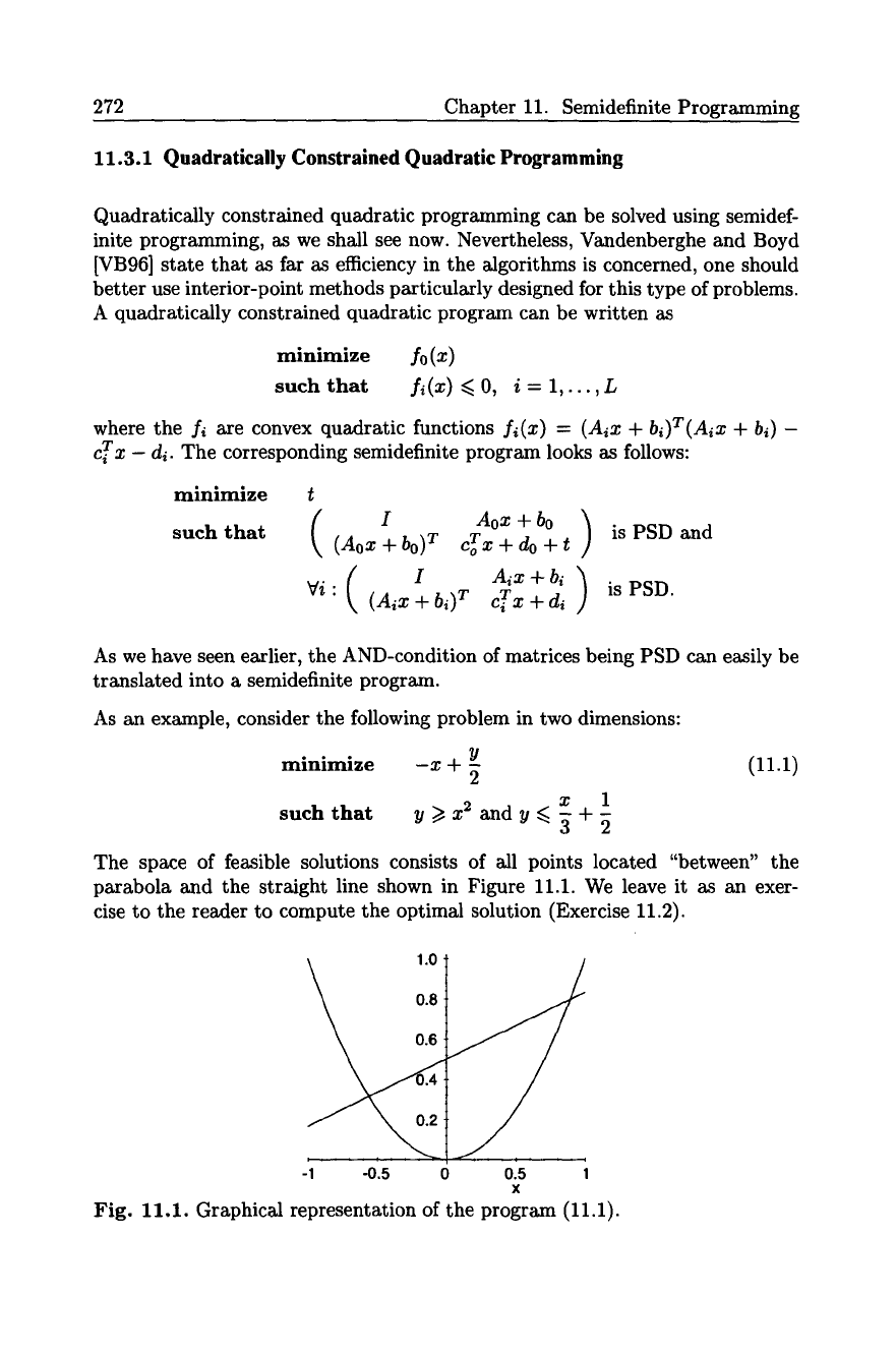
As an example, consider the following problem in two dimensions:
minimize
-x + y
2
x 1
such
that y/>x 2andy~]+
(11.1)
The space of feasible solutions
parabola and the straight line shown in Figure 11.1. We leave it as an exer-
cise to the reader to compute the optimal solution (Exercise 11.2).
consists of all points located "between" the
0.6
J , , , , , ,
-1 -0.5 0 0.5 1
X
Fig. 11.1. Graphical representation of the program (11.1).
11.3. Semidefinite Programming 273
Since the feasible space is convex, we are not able to express a condition like
y ~< x 2 in a semidefinite program. This shows that one has to be careful with
the direction of the inequalities, in contrast to linear programs.
As another example, consider the symmetric 2 • 2-matrix
(:
This matrix is PSD if and only if a >/0, c i> 0, and b z ~< ac. Consequently,
2 x2
allows us to describe the feasible solution space xl 9 x2 ) 4, xl ) 0.
Finally, we remark that in some papers, a semidefinite program is defined by
minimize C 9 X such that
Ai 9 X :
bi (1 ~< i ~< m) and X is PSD
where X, C, Ai are all symmetric matrices. In fact, this is the dual (see Sec-
tion 11.4) of the definition we gave.
11.3.2 Eigenvalues, Graph Theory and Semidefinite Programming
There are interesting connections between eigenvalues and graph theory, let us
for example state without proof the "Fundamental Theorem of Algebraic Graph
Theory" (see, e.g., [MR95b, p. 144]).
Theorem 11.9. Let G = (V,E) be an undirected (multi)graph with n vertices
and maximum degree A. Then, under the canonical numbering of its eigenvalues
Ai for the adjacency matrix A(G), the [ollowing holds:
1. If G is connected, then A2 <
)~1.
2. For l <. i <~ n, lAd ~ A.
3. A is an eigenvalue if and only if G is regular.
4. G is bipartite if and only if for every eigenvalue A there is an eigenvaluc -A
of the same multiplicity.
5. Suppose that G is connected. Then, G is bipartite if and only if -A1 is an
eigenvalue.
274 Chapter 11. Semidefinite Programming
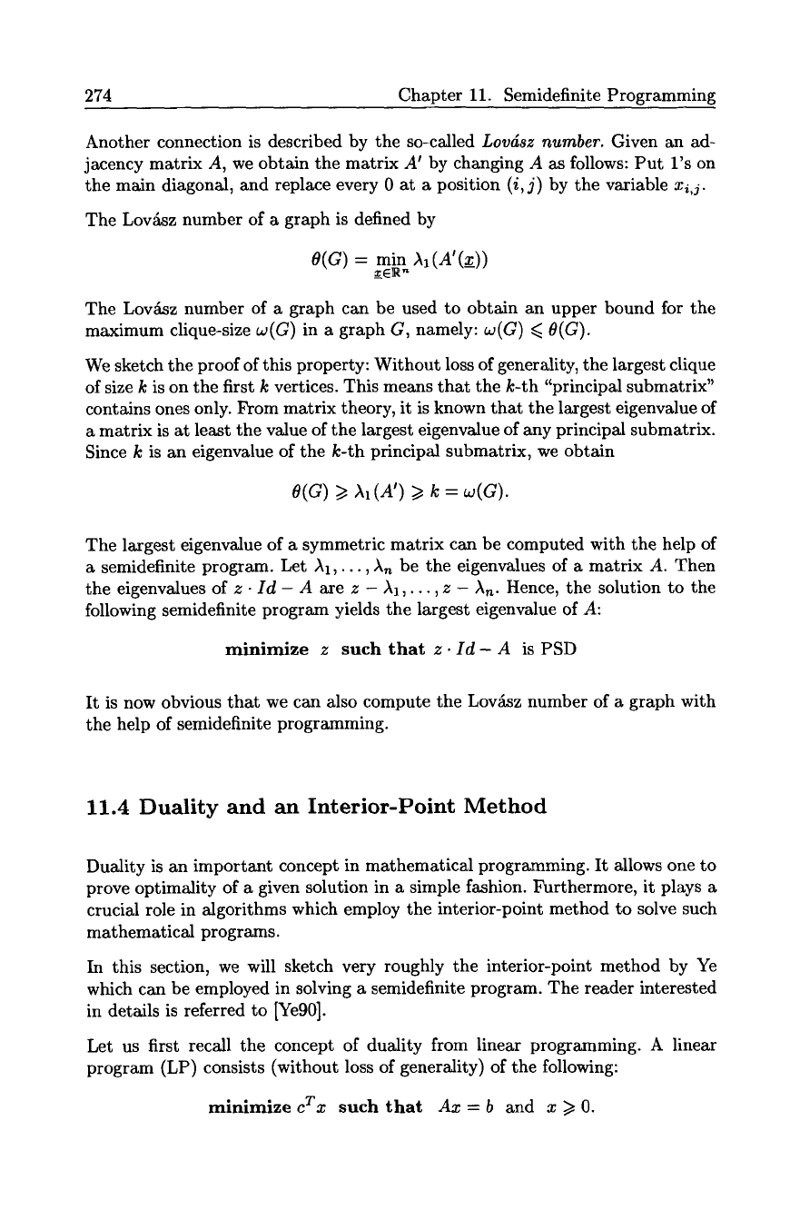
Another connection is described by the so-called
Lovdsz number.
Given an ad-
jacency matrix A, we obtain the matrix A ~ by changing A as follows: Put rs on
the main diagonal, and replace every 0 at a position
(i,j)
by the variable xi,j.
The Lov~sz number of a graph is defined by
O(G) =
min )~1 (A~(x))
x ER '~
The Lov~z number of a graph can be used to obtain an upper bound for the
maximum clique-size
w(G)
in a graph G, namely: w(G) <~
O(G).
We sketch the proof of this property: Without loss of generality, the largest clique
of size k is on the first k vertices. This means that the k-th "principal submatrix"
contains ones only. From matrix theory, it is known that the largest eigenvalue of
a matrix is at least the value of the largest eigenvalue of any principal submatrix.
Since k is an eigenvalue of the k-th principal submatrix, we obtain
O(G) >1 ~1 (A') >/k = wig ).
The largest eigenvalue of a symmetric matrix can be computed with the help of
a semidefinite program. Let )u,..., )m be the eigenvaiues of a matrix A. Then
the eigenvalues of
z 9 Id - A
are z - ~1,.--, z - An. Hence, the solution to the
following semidefinite program yields the largest eigenvalue of A:
minimize
z such that
z 9 Id - A
is PSD
It is now obvious that we can also compute the Lovs number of a graph with
the help of semidefinite programming.
11.4 Duality and an Interior-Point Method
Duality is an important concept in mathematical programming. It allows one to
prove optimality of a given solution in a simple fashion. Furthermore, it plays a
crucial role in algorithms which employ the interior-point method to solve such
mathematical programs.
In this section, we will sketch very roughly the interior-point method by Ye
which can be employed in solving a semidefinite program. The reader interested
in details is referred to [Ye90].
Let us first recall the concept of duality from linear programming. A linear
program (LP) consists (without loss of generality) of the following:
minimize
cTx
such that
Ax = b
and x >/0.
11.4. Duality and an Interior-Point Method 275
As an example,
minimize
Xl
+3x2+x3 such that xl +x2 = 3, x3 -xl = 4,
xl,x2,x3 >~ O.
Without solving the linear program explicitly, we can get bounds from the linear
equalities. For example, since the objective function xl + 3x2 + x3 is at least
x2 +x3, and adding the first two linear equalities yields the condition x2 +x3 -- 7,
we know that the optimal solution cannot be smaller than seven. One can now
see that taking any linear combination of the equalities yields a bound whenever
it is smaller than the objective function. Of course, we want to obtain a bound
which is as large as possible. This yields the following problem.
maximize
b T 9 y
such that
A T 9 y <~ c.
This is another linear program which is called the
dual
of the original one, which
is called the
primal.
Our arguments above can be used to show that any solution
to the dual yields a lower bound for the primal.
This principle is known as
weak duality:
The optimum value of the dual is not
larger than the optimum value of the primal. Even more can be shown, namely
that for linear programming,
strong
duality holds, i.e., both values agree:
If the primal or the dual is/easible, then their optima are the same.
This shows that duality can be used to prove optimality of some solution easily:
We just provide two vectors x and y which are feasible points in the primal and
dual, respectively. If
bTy = cTx,
we know that x must be an optimal point in
the primal and dual problem.
It also makes sense to measure for an arbitrary point x how far away it is from the
optimum. For this purpose, we solve the primal and dual simultaneously. Given
a primal-dual pair x, y in between, one defines the
duality gap
as
e T 9 x - b T . y.
The smaller the gap, the closer we are to the optimum.
Similar concepts hold for semidefinite programming. Before exhibiting what the
correspondences are, we want to sketch how duality can be used in an interior-
point method for solving a linear program.
Khachian was the first to come up with a polynomial-time algorithm for solving
linear programs. His method is known as the
ellipsoid algorithm.
Later, Kar-
markar found another, more practical, polynomial-time algorithm which founded
a family of algorithms known as
the interior-point method.
On a very abstract level, an interior-point algorithm proceeds as follows: Given
a point x in the interior of the polyhedron defined by the linear inequalities,
it maps the polyhedron into another one in which x is "not very close to the
boundaries." Then, the algorithm moves from x to some x ~ in the transformed
space, and it maps x t back to some point in the original space. This step is
repeated until some potential function tells us that we are very close to the