Parinov I.A. Microstructure and Properties of High-Temperature Superconductors

Подождите немного. Документ загружается.

248 5 General Aspects of HTSC Modeling

(5.40), in the case of the boundary rate. We obtain in the boundary mobility

regime, ξ<ξ

, inserting (5.55), (5.58) and (5.59) into (5.39) and (5.40):

−

8F (ψ)ω

3λ(1 − a/l)

; (5.60)



1 −



8F (ψ)ω

3λ(a

)

, (5.61)

where ω = D

1/3

kTγ

is a dimensionless parameter that reﬂects

the ratio of the grain boundary mobility to the pore shrinkage rate by the

grain diﬀusion. The trends in a

/l indicate that solutions exist over a limited

range of ω. For values of ω above a critical value ω

, the absence of a solution

indicates that the shrinkage rate always exceeds the coarsening rate,thatis,the

maximum pore size coincides with initial value, a

. Therefore, pore coarsening

is excluded below a critical pore size, a

∗

, when [1005]

a<a

∗

≈ (7D

1/3

kTγ

)

1/2

. (5.62)

Thus, low boundary mobility and large boundary diﬀusivity are the most

desirable conditions for averting pore–boundary separation.

The densiﬁcation process is accompanied by initial coarsening that causes

a decrease in a/l and an increase in pore size. Therefore, if a/l decreases at

a suﬃciently rapid rate that the transition line ˆa/l is attained, further pore

coarsening is prohibited and the pore shrinkage commences.

When the grain boundary rate is limited by pore drag, the trajectory is

obtained from (5.39), (5.40), (5.56), (5.58) and (5.59) as



1 −

F (ψ)(1 + 3ψ)

3λΔ(1 − a/l)



; (5.63)

=1−



F (ψ)(1 + 3ψ)

3λΔ



1/2

, (5.64)

where Δ = D

. The transition pore size again shows pore coarsening

and shrinkage regions. Coarsening is invariably excluded when the diﬀusivity

ratio and dihedral angle satisfy the condition:

> 3λ/F (ψ)(1 + 3ψ) . (5.65)

Otherwise, there is no maximum, and pore coarsening inevitably initiates

whenever a/l becomes smaller than a

/l. Both considered regimes of grain

growth can be generalized as it is shown in Fig. 5.20. Recognizing that the

transition pore sizes pertinent to the individual grain growth regimes will typ-

ically intersect, this intersection may be found by using inequalities (5.62) and

(5.65). When both inequalities are closely approached, the intersection occurs

within an intermediate range of a/l(∼ 0.2–0.3), and exclusion of pore coars-

ening is contingent upon less stringent conditions than suggested by either

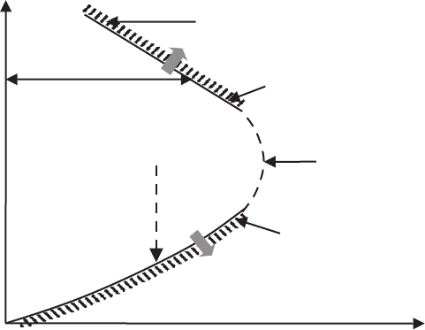
5.2 Void Transformations During Sintering of Sample 249

Pore Coarsening

Pore

Shrinkage

Pore Drag Limited

Coarsening

Boundary Mobility

Limited Coarsening

Pore Coarsening

Excluded

•

Trajectory

a, M

1/3

F(Ψ)/kT γ

a/l

Fig. 5.20. A schematic illustration of the general tendencies in the transition

pore size

inequality (5.62) or inequality (5.65) (Fig. 5.20). Otherwise, the coarsening

behavior is dominated either by pore drag or by the grain boundary mobility.

The intersection is caused by the initial pore size, the grain boundary mo-

bility and the surface diﬀusivity. In particular, small values of a

and

simultaneously induce intersection behavior, narrowing the region of pore

coarsening.

The pore coarsening value outside the exclusion region can be deduced,

in principle, by superimposing onto Fig. 5.20 the line that indicates the tran-

sition from pore drag to grain boundary mobility limited grain growth and

evaluating the coarsening that occurs in each region. An upper bound pore

size, when it exists, has a functional form [1005]:

ˆa/l = F

kT/D

(ψ

−1

) , (5.66)

where F

are increasing functions of the pertinent variables.

5.2.3 Estimation of Pore Separation Eﬀects for HTSC

The coarsening parameter that exerts a major inﬂuence on the ﬁnal mi-

crostructure is the peak pore size, ˆa (see Fig. 5.21). Its comparison with the

critical pore size, a

, deﬁned by (5.34), states its breakaway from grain bound-

ary. The pore-breaking behavior is caused primarily due to the pores in triple

junctions (and pores with this morphology dominate the peak pore size, ˆa). At

the same time, only those pores at two-grain interfaces are amenable to separa-

tion from grain boundaries [445] (at pore sizes >a

). Thus, in the comparison

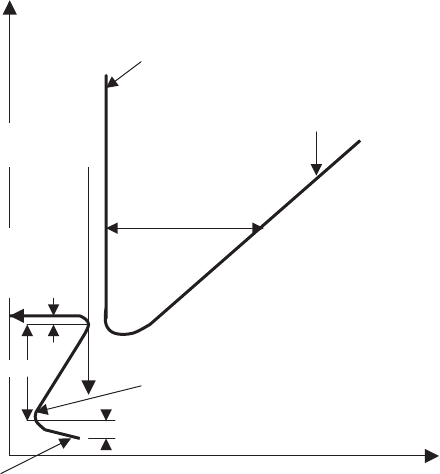
250 5 General Aspects of HTSC Modeling

Pore Radius

Small Grain Diameter

Initial

Compact

Pore/Grain

Trajectory

Coarsening

Shrinkage

and Final

Densification

Pore Size

Maximum, a

Separation

Geometric

Limitation

Lower Bound

Critical Pore Size, a

Rearrangement

•

Fig. 5.21. The relation between critical pore size for separation,a

, and peak pore

size, ˆa

of ˆa and a

, it is necessary to assume the concurrent existence of pores of sim-

ilar dimensions on both two- and three-grain interfaces. Non-separating pores

on two-grain interfaces become inevitably attached to three-grain corners dur-

ing small grain disappearance [445] that leads to subsequent enlargement by

pore coalescence. A part of the coarsened pores may subsequently translate

again onto two-grain interfaces causing the process to repeat until either the

peak size is reached or the pores on two-grain interfaces become large enough

to separate.

Comparing (5.3) and (5.66), the understanding for the possibility of avert-

ing pore separation in small microstructures is provided, for which pore shrink-

age and pore motion are dominated by grain boundary diﬀusion and surface

diﬀusion, respectively. Note that requirements of small grain-boundary mobil-

ity and large grain-boundary diﬀusivity are evident. However, these conditions

can only be simultaneously satisﬁed in the presence of appreciable solute (or

precipitate) drag throughout the grain disappearance process. Hence, a vi-

tal inﬂuence of drag-inducing solutes upon the attainment of optimum mi-

crostructures is apparent.

The trends connected with the surface diﬀusion can be stated for two ex-

tremes, namely (i) when a

>> a

∗

pore breakaway can be avoided

by increasing the ratio of the boundary to surface diﬀusivity, consistent with

5.3 HTSC Microstructure Formation During Sintering 251

condition of a

, until (5.65) is satisﬁed. This trend is entirely compatible

with that needed to achieve densiﬁcation during the initial stage of sintering

[126, 414]. Conversely, in the case (ii) when a

∼ a

∗

, large values of the surface

diﬀusivity are needed to ensure that a

>aduring subsequent pore coarsen-

ing [414]. This requirement is distinctly diﬀerent from the initial stage of

densiﬁcation. Hence, diﬀerent temperatures are undoubtedly desirable during

the initial and ﬁnal stages of sintering. Also note that the explicit statement

of diﬀerent thermal treatments depends on the values and temperature de-

pendencies of both the surface and boundary diﬀusivities and also the grain

boundary mobility.

The presented analysis of pore transformation as a result of grain growth,

based on the surface diﬀusivity mechanism, is well satisﬁed for ﬁne pores.

Transformations of larger pores, when their motion is caused by the diﬀerence

of the leading and trailing surface curvatures, can be also studied, taking

into account corresponding changes of gas pressure in diﬀerent points of the

pore surface [443]. This case is less interesting for HTSC and therefore is not

considered here.

Finally, (5.34) is used for quantitative analysis of possible pore sizes, which

break away from grain boundaries during sintering of monocore Bi-2223/Ag

tapes. Selecting required parameters as follows [670, 671, 864]: Ω =2.2 ×

−30

, D

=2.5 × 10

−21

/c, γ

=2γ

, ψ

max

= π/2,T = 1110 K, 2R =

25 μm,k =1.38 ×10

−23

J/K (here the some parameters is selected for Al

because corresponding data is absent for Bi-2223), we obtain a very high value

of M

≈ 4 × 10

m/(N · c) even for a

= 100 nm. For smaller pores separated

from grain boundary, longer grain mobility is required. Obviously, the size of

pores, which can be separated from grain boundaries during prolonged an-

nealing, on some orders of magnitude is longer than the coherence length

(∼ 1 nm) in Bi-2223. Therefore, these separated pores cannot serve eﬀective

pinning centers and because of percolation features must considerably dimin-

ish the critical current. Apparently, in prolonged annealing, this eﬀect is more

important than deteriorating pinning strength due to lead expelling [670, 671].

We think that namely numerous pore separations and their movement into

grain insides have found the critical current decrease in longer calcining after

observed I

maximum at about 180 hs annealing of monocore Bi-2223/Ag

tapes [670, 671]. Thus, the lead expelling causes a decreasing of critical cur-

rent in long reaction, but rather due to pore transformations, occurred during

annealing (because Pb can inhibit only a local grain growth in this case), than

thanks to decrease of its pinning eﬃciency in the grains.

5.3 HTSC Microstructure Formation During Sintering

For investigating the processes of HTSC ceramic preparation, plane sample

of superconducting powder compact in gradient furnace is considered. Two-

scale modeling, consisting of the macroscopic study of the precursor powder

252 5 General Aspects of HTSC Modeling

sintering and microstructure formation into the region of the heat front prop-

agation is carried out. For this, the considered rectangular region [a, b]is

divided into square lattice with characteristic size of elementary cell, δ,which

corresponds to either particle or pore. The sample moves into gradient fur-

nace with constant rate, v (which can be correlated with the temperature

change rate of the sample surface). Moreover, it is assumed that temperature

distribution T into furnace depends on one coordinate x and consists of sites

with constant temperature and linear dependence on this coordinate. In order

to solve an initial-boundary problem, the method of summary approximation

(MSA) is used (see Appendix C.1).

Microstructure modeling begins from the pore generation in the initial

sample by using Monte-Carlo procedure. In this case, it is suggested that

the pores are distributed in accordance with the normal distribution, and

pore start concentration (i.e., porosity) C

is given in diﬀerent variants of the

computation. This procedure can be carried out, for example, ﬁlling the cells

of the initial lattice by arbitrary numbers, using the generator of arbitrary

numbers (GAN) and then selecting a number of minimum values that corre-

sponds to the pore number. In order to obtain the statistically reliable results,

the computations are accompanied by averaging of the pores and crystallites

distributions in the sample microstructure.

The model includes the following main stages, namely (i) a heat front dis-

placement and deﬁnition of the material sintering region; where a temperature

above the sintering temperature, u

; (ii) a press-powder re-crystallization into

the corresponding region; and (iii) a shrinkage of the microstructure formed.

The ﬁrst from pointed steps relates to the macroscopic modeling and the other

two to the microscopic modeling.

The computation of eﬀective heat conduction (see Appendix C.2) for non-

sintered part of the sample consists of the following stages. First, a coor-

dination number, N

, and the sizes of element with averaged parameters

) using (C.2.12), (C.2.22) and (C.2.28) is deﬁned. In order to calcu-

late the heat conduction of gas into gaps between particles, δ

, λ

and λ

from (C.2.37), (C.2.35) and (C.2.34) are computed successively. Then, the

heat conduction of frame is computed depending on the porosity of the con-

sidered region, using (C.2.43). The porosity of the second-order structure

is computed on the basis of (C.2.17) and then, using (C.2.5) and (C.2.6),

= c is calculated. In this case, the heat conduction of gas into pores of

the second-order structure, λ

, is deﬁned, using (C.2.20). Finally, the ef-

fective heat conduction of the non-sintered part of the sample is calculated

using (C.2.13).

In order to study a displacement of the thermal front, the ﬁrst main prob-

lem for quasi-linear equation of heat conduction with a variable u = T − T

is considered, where T

is the environment temperature:

∂u

∂t

∂

∂x



k(u, C

)

∂u

∂x



∂

∂y



k(u, C

)

∂u

∂y



, (5.67)

5.3 HTSC Microstructure Formation During Sintering 253

with initial condition

u(0,x,y)=0, (5.68)

and boundary conditions

u(t, 0,y)=u

(t); u(t, a, y)=u

(t); u(t, x, 0) = u(t, x, b)=u

(x, t) .

(5.69)

Here, k(u, C

) is the temperature conductivity factor; and C

is the pore

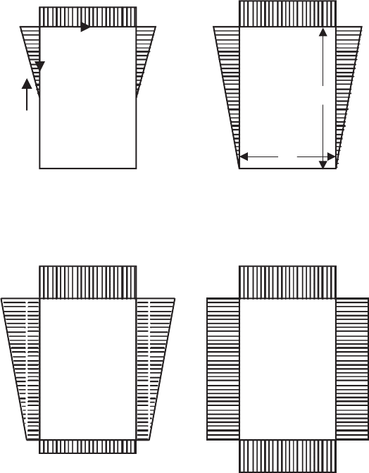
concentration or porosity. The boundary conditions are shown schemati-

cally in Fig. 5.22 for diﬀerent time, t. In this case, the function u

(x, t)has

the form:

(a) u

(x, t)=



(vt−x)

x ≤ vt

0 x>vt

, (5.70)

(b) u

(x, t)=A

(a − x)

;(c)u

(x, t)=u

max

− u

)(a − x)

(5.71)

where A

is the given constant. The calculation is ﬁnished in the case of

reaching in the whole region the temperature, u(x, y) ≥ u

The boundary conditions (5.69)–(5.71) correspond to a scheme of the ce-

ramic gradient sintering [516]. In the case of hot-pressing, these boundary

conditions are replaced by the following ones [823]:

u(t, 0,y)=u(t, a, y)=u(t, x, 0) = u(t, x, b)=A

t. (5.72)

In the beginning of the modeling, preliminary, the start porosity, C

,the

sintering temperature, u

max

(where u

max

is the maximum temperature

into gradient furnace for considered site of sintering) and the sample move-

ment rate, v, are assumed to be known. The temperature conductivity factor

at the ﬁrst stage is found by constant values of heat capacity, c

,andmaterial

density, ρ, and also by heat conduction factor, λ, depending on press-powder

porosity. As λ is selected a value of the heat conduction factor, λ

,iscalcu-

lated on the basis of the generalized conductivity principle (Appendix C.2).

Hence, k(u, C

)=λ

/(c

ρ).

A solution of the problems (5.67)–(5.71) is obtained on the basis of

the method of summary approximation (MSA) by using pure non-evident

local one-dimensional scheme (LOS) (Appendix C.1). For this aim, a ﬁnite-

diﬀerence counterpart of the initial-boundary problems (5.67)–(5.71) is writ-

ten. The ﬁnite-diﬀerence equation is solved, using the run method. In order

to obtain the required temperature ﬁeld at any step of the considered pro-

cess, there is a non-linear equation solved by iterations. After deﬁnition of

temperature distribution into region, where u ≥ u

, a modeling of the mate-

rial re-crystallization and shrinkage is carried out. Note that the grain formed

at any stage can penetrate into earlier “sintered” region if it is allowed by

the microstructure porosity. After that, the heat conduction factor is altered

254 5 General Aspects of HTSC Modeling

= A

= u

max

u = u

max

= A

= 0

= u

= 0

(a)

(b)

Fig. 5.22. Change of boundary conditions during heating of the sample

and the corresponding value of the temperature conductivity factor is calcu-

lated. At the every stage of the microstructure modeling, λ

will be deﬁned

by the heat conduction of sintered and non-sintered regions. The ﬁrst re-

gion possesses heat conduction of fabricated material. At the same time, this

parameter is calculated for non-sintered region taking into account an exist-

ing porosity by using the generalized conductivity principle (Appendix C.2).

Therefore, λ

in the whole considered region is deﬁned by concentration of

both components and by the values of their heat conduction by using the

rule of mutual-penetrating components (see (C.2.13)). Then, a transition to

the next time interval is carried out. The process ﬁnishes after microstructure

5.3 HTSC Microstructure Formation During Sintering 255

formation in the whole considered region, which, as a result, consists of pores

and grains.

Separately, the microstructure mechanisms of the superconducting press-

powder re-crystallization and shrinkage for the formed structure in the

temperature region, u ≥ u

, are modeled. The process of the crystallite nu-

cleation into precursor press-powder is assumed to be the thermal activated

process. Therefore, an arbitrary number corresponds to each remaining (after

modeling of porosity) cell of the considered region. This arbitrary number

characterizes the initiation time of a single crystallite, and these numbers

are obtained by using GAN from the law of exponential distribution [1002]:

(t)=1− exp(−t/τ

), where τ

∼ exp(U/ku

) is the mean expectation

time of the crystallite nucleation in the node of i-line and j-column; U is

the activation energy of crystallite nucleation; k is Boltzmann constant; u

is the temperature in the lattice cell with coordinates (i, j). It is suggested

that a crystallite with minimum nucleation time, t

∗

, ﬁrst nucleates, and its

nearest neighbors with coordinates (k, l) obtain priority. According to this,

the values of t

are decreased. At the next step, a minimum nucleation time,

∗

, is again found among of all remaining lattice cells, and a new crystal-

lite nucleates in the corresponding cell. This cell is either the nearest cell to

the earlier-nucleated crystallite or far from it. In the ﬁrst case, there is a

grain growth in the re-crystallization process. Generally, the nucleation time

of crystallite, t

, near with earlier-nucleated one is deﬁned as

∗

− t

S exp(1 − S)

, (5.73)

where S is the grain square (which is deﬁned by the corresponding number

of cells) near of that it is possible an nucleation of a new crystallite. Note that

relation (5.73) causes a decreas of the nucleation time of neighbor cells, until

S is suﬃciently small, and the time increases together with the grain area due

to pushing of secondary phases at the intergranular boundaries during grain

growth.

After completion of the crystallite system formation into region of or-

der of the sintering front width, a shrinkage of the sample is modeled. One

includes pushing of gaseous component from the sample and decreasing of

closed porosity, thanks to grain movement. Computational algorithm of the

shrinkage provides successive alternating displacements of grains along two

orthogonal directions upon total exhaustion of possibility of their movement.

In the displacement process, it is assumed that grains preserve own volume,

shape and spatial orientation. This is achieved due to successive deﬁnition

for each lattice layer of possibility of the grain movement (this considered

grain consists of single cells) and its displacement as a single whole. In the

calculation, it is assumed that the shrinkage process occurs instantaneously.

The completion of the grain structure formation during the re-

crystallization and shrinkage is accompanied by beginning of secondary

re-crystallization, that is, abnormal grain growth due to existence of the pores

256 5 General Aspects of HTSC Modeling

and admixture phases. This grain growth occurs at maximum pressure and

a linear character of the temperature change (0 ≤ T ≤ T

max

,whereT

max

the maximum temperature into furnace) [1034]. The modeling of the abnor-

mal grain growth is carried out on the basis of the Wagner–Zlyosov–Hillert’s

dynamic growth models [1, 2, 245].

5.4 Microcracking of Intergranular Boundaries

at Sample Cooling

A plane sample of sintered ceramic into gradient furnace is considered. After

sintering, a uniform temperature, u = u

max

, is stated in the whole sample.

Due to a shrinkage during the sample cooling, the rectangular site of the front

with sizes a

≤ a and b

≤ b is considered, which excludes the layers, includ-

ing only elements of open porosity. At macroscopic modeling of the cooling,

it is assumed that heat conduction factor is found by the thermal conduction

of the sintered material and depends only on temperature, u. The modeling

of the heat front movement continues down to attainment of room tempera-

ture at one of the sample boundaries. Because intergranular boundaries (the

main stress concentrators in this case) are subject to cracking at cooling, the

required values (i.e., temperatures and stresses) are calculated in the lattice

nodes but do not in the lattice cells, as in the case of sintering.

A modeling of microcracking consists of the following stages: (i) a displace-

ment of heat front and deﬁnition of temperature ﬁeld, (ii) a calculation of nor-

mal thermal stresses in the lattice nodes, (iii) a division of all intergranular

boundaries into separate sections, (iv) a computation of mean normal stress,

acting onto given section and (v) a satisfaction to microcracking condition.

Similar to the problem of ceramic sintering, it is assumed that the sam-

ple displaces with constant rate, v (which can be also correlated with the

temperature change rate of the sample surface), from gradient furnace. The

temperature changes in linear law into furnace. In the calculation of temper-

ature ﬁeld, the initial-boundary problem (5.67)–(5.69) is considered, where

initial condition reduces to u(0,x,y)=u

max

, and boundary conditions are

depicted in Fig. 5.23. In this case, a function u

(x, t)isgivenas

(a) u

(x, t)=u

max

; (5.74)

(b) u

(x, t)=



max

−u

max

)

(vt − x) x ≤ vt

max

vt ≤ x ≤ a

, (5.75)

As a result of the solution of this thermal conduction problem, a tem-

perature distribution, causing corresponding thermal stresses, is calculated.

Similar numerical algorithm may be applied to modeling of microcracking pro-

cesses during cooling of oxide superconductor from room temperature down to

cryogenic one its application.

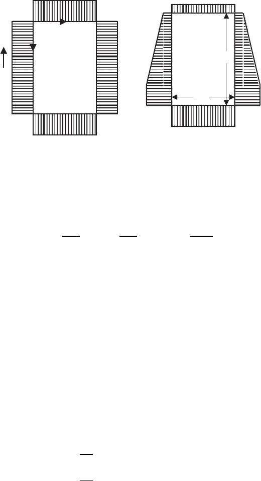
5.4 Microcracking of Intergranular Boundaries at Sample Cooling 257

u = u

max

= u

max

≤ u

< u

max

(a)

(b)

Fig. 5.23. Boundary conditions for problem of sample cooling

In order to deﬁne 2D stress state, the method of ﬁnite diﬀerences [663] is ap-

plied. For framework of the thermal stresses problem, stress state is calculated

through Airy’s function, ϕ

∂

∂y

; σ

∂

∂x

; σ

= −

∂

∂x∂y

. (5.76)

In this case, the function ϕ satisﬁes the diﬀerential equation in partial

derivations:

ϕ + EαΔu =0, (5.77)

where Δ = ∂

/∂x

+ ∂

/∂y

;Δ

= ∂

/∂x

+2(∂

/∂x

∂y

)+∂

/∂y

; Eα =

const; E is Young’s modulus; α is the thermal expansion factor and u = u(x, y)

is the temperature, calculated from a some value, in which the thermal stresses

are absent.

Replacing the partial derivations in (5.77) by ﬁnite diﬀerences, we obtain

for arbitrary point 0 of the considered region (Fig. 5.24):

20ϕ

− 8(ϕ

+ ϕ

)+2(ϕ

+ ϕ

+(ϕ

+ ϕ

)+Eαδ

+ u

− 4u

)=0. (5.78)

In the case of simply connected region and absence of external loading,

the boundary conditions can be presented as [1062]

ϕ =

∂ϕ

∂y

=0 atx =0;x = a

; (5.79)

ϕ =

∂ϕ

∂x

=0 aty =0;y = b

. (5.80)

The conditions (5.79) and (5.80) sign a deﬁnition of zero values of principal

vector and principal moment of the acting forces at the region boundaries.