Roy K.K. Potential theory in applied geophysics
Подождите немного. Документ загружается.

17.1 Introduction 569
(a)
(b)
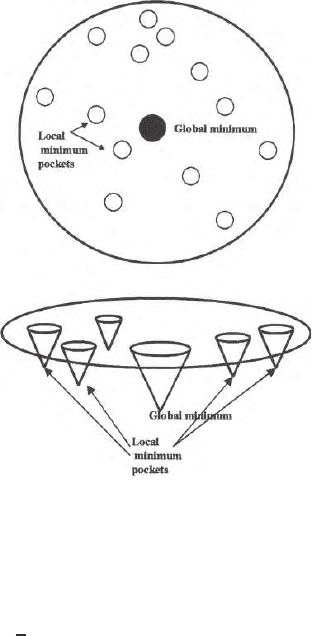
Fig. 17.7. a, b. Local minima po ckets in the parameters space; these are model
traps, prevent the models from further movement towards global minimum
distribution. Principle of equivalence in electrical and el ectromagnetic the-
ory tells that for different combinations o f layer resistivity and thickness one
gets T(= hρ) and S(=
h
ρ
) equivalence where ρ is the resistivity and h is the
thickness of a layer in a n one dimensional layered earth problem.
Since retrieval of a model from a set of data is to see the different projec-
tions of the model in the Hilbert space from different angles, data inadequacy
will increase the non uniqueness due to partial view of the model from different
projection angles.
Noise in the field data is an inevitable process. Noise will be there in the
data collected from the field. Higher noise level can completely vitiate inverse
process. Opacity increases in the observation power of the data. So the model
space can be either empty (null information) or infinite dimensional (Bachus
and Gilbert 1967).
Varied initial choices and presence of many loc al minima pockets bring
non un i queness in an inverse problem. From different points in the space
when the initially assumed models start moving, they get trapped at different
local minima and generate different answers. Therefore judicious initial choice
of the model parameters is essential to reduce the starting distance between
m
Prior
and m
true
where m
true
is the true model parameter. In that case this
probability to get trapped in local minimum reduces. Interpreter should cho ose
570 17 Inversion of Potential Field Data
the initial model with available known geology of the area. Difference in the
choice of forward model will generate different answers. It is interesting to
note that the interpreter often over parameterises the model to make i t an
underdetermined problem and get interpretable encouraging results. Even if
the initial forwar d mo del is totally a wrong choice and do es not have any
closeness with the loca l geology, on e may get both convergence and stability
of an inverse problem and get an answer. This is a note of caution. The
convergence i.e., the reductions of the discrepancy between the field data
and the model data in successive iteration does not guarantee any acceptable
result. Interpreter should have some knowledge about the local geology of the
area to get a meaningful results.
A class of inverse problems which use differential op erators are generally
made linear by truncating higher order terms of the Taylor’s series expa nsion
of non li n ear problems. This approximation may b e too severe for a certain
class of strongly nonlinear prob lems. This linearisation, coupled with limited
resolving power of the potential problems, inadequate and inaccurate data
generate non uniqueness. Interpreter dependent factors are the (i) nature of
smoothness used in data processing (ii) choice of a particular approach for
inversion (iii) differe nt way of discretisation to generate data. (iv) use of dif-
ferent softwares.
Even with all these problems of non uniqueness if we have good quality
adequate data, one can get a cluster of models in the parameter space or M-
space near the actual answer. If several earth models obtained using different
approaches of inversion have some common feature then earth must have that
property (Bachus a nd Gilbert 1967). Thus inverse theory survives with con-
siderable success while imaging extremely complicated, inhomogeneous an d
anisotropic earth even in this high level of non uniqueness.
17.2 Wellposed and Illposed Problems
The concept of well posed and ill posed problems were introduced by
J. Hadamard (1902, 1932) in an attempt to classify the different types of
differential equations along with their boundary conditions.
A solution is said to be well posed for solution of the equation
Az =u
n × mm× 1n× 1
(17.1)
where the initial choice of model parameter z is in the model space M and u is
in the data space D. These spaces are M and N dimensional abstract spaces.
These spaces are metric spaces, Euclidean space, pre-Hilbert space, Hilbert
space, normed inner product space etc(Sect. 17.4).
A problem of determining a solution z in the space M from the initial data
u in the D space is well posed o n these spaces (D and M) if the following
condition are satisfied:
17.4 Abstract Spaces 571
a. For every element u ∈ D, there exists a solution in the M space
b. The solution is unique
c. The solution is stable on the spaces D and M
Problems that do not satisfy these conditions are termed illposed problems.
Most of the geophysical problems are illpo sed because the data are noisy and
as a result there can be infinitely ma ny solutions which will satisfy all the
data.
17.3 Tikhnov’s Regularisation
If a small perturbation in the data generates a small perturbation in the model
parameters and vice versa th en the inverse problem is a stable but not nec-
essarily well posed .If a minor change in the data invites major change in
the model the prob lem is definitely an ill posed problem. Regularisation in
the data may be necessary to an ill posed problem and to get an approxi-
mate solution which is stable. It may be based on providing supplementary
information from completely independent sources. An attempt is being made
to construct an approximate solution of (17.1), that are stable under small
changes in the data space through use of a regularization op erator. With noisy
data set u
δ
, the approximate model set is Z
α
=R(u
δ,
α), obtained with the aid
of regularizing operator R(u,α)whereα = α(δ, u
δ
). Here δ is th e noise level.
α is the regularizing parameter. Every regularizing parameter defines a stable
metho d of approximate construction of a solution of (17.1). The choice of the
regularizing parameter(s) should b e consistent with the a ccuracy of assess-
ment of δ the noise level in the data (α = α(δ). This regularizing parameter
α is chosen in such a way that when δ → 0andu
δ
→ u then Z tends towards
Z
T
or Z
true.
. Thus the problem of finding an approximate solution of (17.1),
is centered around getting a stable solution under minor perturbation in the
data space and determining the regularization parameter α from additional
information related to the problem. This method of constructing the approxi-
mate solution i s called the regularization method. This is the basic philosophy
of Tikhnov’s Regularisation( Tikhnov and Arsenin 1977).
All kinds of data smoothing, Occam’s rajor, generation of minimum struc-
ture algorithm, intro duction of different kinds of constraints, application of
data and model variance-covariance matrices for bringing stability in an inver-
sion algorithm are the members of the regularization club.
17.4 Abstract Spaces
17.4.1 N–Dimensional Vector Space
A vector is a collection of n real numbers a
1
......... a
n
in a definite
order where n is any integer. This vector is a = (a
1
............a
n
)where

572 17 Inversion of Potential Field Data
a
1
..........a
n
are the components of the vector ‘a’. Two vectors ‘a’ and ‘b’
are equal if a
i
=b
i
for i = 1 ...........n.
These vectors in an n-dimensional space fulfill certain algebraic laws.
These are
(i)
(a + b) = (b + a)(associativity law of addition) (17.2)
(ii)
(a + b) + c = a + (b + c)(distributive law) (17.3)
(iii)
λ(a + b) = λa+λb(multiplication law) (17.4)
where λ is a scalar.
(iv)
λ(µa) = (λµ) a(asso ciativity law of multiplication) (17.5)
(v)
0a = θ(concept of null vector). (17.6)
where θ is a zero or null vector. A real space in space domain can have 3
dimensions. We often bring the concept of 4th dimension bringing time or fre-
quency into consideration. But when we try to conceive of a space for a set of
geophysical data collected on the surface of the earth, we think of an n dimen-
sional data space and an m dimensional parameter space. ‘n’ will depend upon
the number of data collected and ‘m’ depends on the parameters that can be
retrieved from the information collected. Variation of the physical properties
and their dimensions in the space domain generate m number of model param-
eters. These data and model parameters generate D and M vector spaces.
17.4.2 Norm of a Vector
Length or norm of the vector ‘a’ in ‘R’ is the arithmetic square root of sum
of the square of the components. The norm of a vector ‘a’ is denoted by ||a||
and is given by
||a|| =
a
2
1
+a
2
2
+a
2
3
+ .......a
2
n
(17.7)
If coordinate of a point P is (x, y, z) in a three dimensional space, its distance
from the origin (0, 0, 0) is d =
x
2
+y
2
+z
2
. Therefore (17.7) is an n dimen-
sional generalisation of 3 dimensional real space concept of distance or norm.
The prop erties of norm are
(i)
||a|| ≥ 0for all a and||a|| = 0 (17.8)
only if a = θ.
(ii)
||λa|| = |λ|||a|| (17.9)
17.4 Abstract Spaces 573
(iii)
||a+b|| ≤ ||a||+ ||b||. (17.10)
An n–dimensional vector space R in which norm of a vector is defined is called
an n–dimensional Euclidean space. A vector with an infinite set of components
in an infinite sequence of real numbers (a
1
, a
2
,....a
∞
) is an infinite dimen-
sional Euclidean space.
17.4.3 Metric Space
A metric space is an n dimensional abstract space where a non-negative real
number called distance is defined between any two elements of a
1
and a
2
and
is denoted by d(a
1
, a
2
). It satisfies the following conditions, i.e.,
(i)
d(a
1
, a
2
)=0 ifa
1
=a
2
(17.11)
(ii)
d(a
1
, a
2
)=d(a
2
, a
1
) (17.12)
(iii) for any thr ee elements of the abstract space.
d(a
1
, a
2
) ≤ d(a
1
, a
3
)+d(a
3
, a
2
) (17.13)
(iv) d(a
m
, a
n
) → 0forn,m→∞
17.4.4 Linear System
A set of vectors S forms a linear system if the concept of additions and mul-
tiplications are satisfied as shown in (17.2 and 17.4).
17.4.5 Normed Space
A linear system ‘a’ is called a normed space if for every element a
n
in S,
a real nu mber called norm is defined. Normed space will have the following
properties.
(i)
||a|| ≥ 0 for any a ∈ S (17.14)
(ii)
||a|| =0 fora=θ (17.15)
(iii)
||λa|| = |λ|||a|| (17.16)
for any a ∈ S and for any scalar number λ.
(iv)
||a+b|| ≤ ||a||+ ||b|| or any a, b ∈ S (17.17)
574 17 Inversion of Potential Field Data
(v)
d(a, b) = ||a − b||, (17.18)
the distance in a normed space.
(vi)
||a|| = ||a − θ|| =d(a, θ), (17.19)
i.e., the norm of any element is its distance from the origin.
17.4.6 Linear Dependence and Independence
Elements a
1
, a
2
......a
n
∈ S are called linearly independent, if for a linea r
combination o f these elements, the relation Σλ
k
a
k
= θ is satisfied only for λ
1
=
λ
2
= λ
3
......λ
n
= 0. Otherwise the elements ar e called linearly dependent.
Elements a
1
, a
2
,.....a
n
are linearly dependent if and only if, at least one of
them can be expressed in the form of a linear combination of the others.
If an elements a ∈ S can be expressed in the form of a linear combination
of linearity independent elements a
1
,a
2
,a
3
.....a
n
,anda=
n
4
k=1
λ
k
a
k
,thenλ
k
will have unique values. These normed space are finite dimensional.
17.4.7 Inner Product Space
Suppose a = (a
1
, a
2
,....a
n
)andb=(b
1
, b
2
, b
3
....b
n
) are vectors in the
space R. The dot product or inner product of the two vectors are defined by
(a, b). It is defined to be the scalars obtained by multiplying corresponding
components and adding the resulting products.
u.v =
n
k=1
u
k
.v
k
(17.20)
17.4.8 Hilbert Space
Let the space S b e a real linear system and suppos e that in any two of its
elements a, b there exists a real number denoted by (a, b) and also possess
the following proper t ies
(i)
(a, b) = (b, a) (17.21)
(ii)
(a + b, c) = (a, c) + (b, c) (17.22)
(iii)
(λa, b) = λ(a, b) (17.23)
(iv)
(a, a) = 0if and only if x = θ (17.24)

17.5 Some Properties of a Matrix 575
(v)
||a|| =
(a, 0). (17.25)
A complete normed real space in which the norm is generated by the inter
product or scalar product is called a Hilbert space.
Abstract spaces in Inverse Theory, viz. data space a n d model space follow
the properties of these Eucledean space, Metric space, normed linear space,
Inner product space and Hilbert space. Further detail s are beyond the scope
of this volume.
17.5 Some Properties of a Matrix
17.5.1 Rank of a Matrix
Many of the physical problems in their final stages of formulation reduce to a
matrix equation in the form
Ax = B (17.26)
where A is an n×m known matrix, B is a known vector of n elements and x is
an unknown vector of m elements. We have to consider whether there exists
a vector x which satisfy this equation an d whether the set of simultaneous
equations which satisfy (17.26) is consistent. The answer is provided by rank
of the matrix ‘A’. ‘n’ elements f
1
, f
2
, f
3
............f
n
of a linear space R are
linearly dependent if there exists C
j
∈ F not all equal to zero, such that
n
j=1
C
j
f
j
= 0 (17.27)
otherwise they are linearly independent. The rank of a matrix is equal to the
number of linearly independent equations and the number of nonzero eigen
values present in the system. The order of the largest non-zero minor is also
the rank. Theoretically, if rank of a matrix is equal to the number of unknown
parameters m, the solution should be unique if it exists. For practical problems
that is not possible because the data are noisy.
If the rank of the matrix is k and the system of equations is consistent,
then we shall have six possible cases, i.e.,
(i) n=m and k=m
→ Even determined problem
(ii) n = m and k < m
(iii) n > mandk=m
→ Over determined problem
(iv) n > mandk< m
(v) n < mandk=n
→ Underdetermined problem
(vi) n < mandk< n
576 17 Inversion of Potential Field Data
where n is the numb er of data points in D-space and m is the number of
parameters in M-space. k will a lways be either equal to or less than m or n
which ever is less. n > m does not guarantee that the problem has become
an overdetermined problem. The capability of data to see a target completely
must be taken into consideration. Similarly one can make an overdetermined
problem under determined by overparameterising the models. Sometimes it
gives more realistic r esult sp ecially in one dimensional problems.
17.5.2 Eigen Values and Eigen Vectors
Determine a scalar quantity λ and a vector U which satisfies (17.2). This
equation can be expre ssed in the polynomial form as
λ
n
+C
n−1
λ
n−1
+ .........+C
1
λ = 0 (17.28)
The n ro ots of this p olynomial
λ
1
, λ
2
, λ
3
.........λ
n
are the eigen values of the system matrix. They satisfy the equations
Au
i
= λ
i
u
i
(17.29)
where u
i
is called the eigen vector. The set of eigen values form a diagonal
matrix and is called the spectrum o f A. The largest absolute value of λ is
called the spectral radius. Every eigen value has a eigen vector. It is a column
vector. Even a zero eigen value has a non zero column eigen vector.
An n × n square matrix has at least one and at the most n distinct eigen
values. We can write (17.29) as
a
11
x
1
+ ...............+a
1n
x
n
= λ
1
x
1
a
21
x
1
+ ...............+a
2n
x
n
= λ
2
x
2
‘
‘
a
n1
x
1
+a
n2
x
2
...............+a
nn
x
n
= λ
n
x
n
. (17.30)
By transferring the right hand column to the left hand side we get
(a
11
− λ
1
)x
1
+a
12
λ
2
+ ...............+a
1n
x
n
=0
a
21
x
1
+(a
22
− λ
2
)x
2
+ ...............+a
2n
x
n
=0
‘
‘
a
n1
x
1
+a
n2
x
2
...............+(a
nn
− λ
n
)x
n
= 0 (17.31)
Number of non zero eigen values dictates the quality of t he matrix, for starting
an inverse problem.
17.5 Some Properties of a Matrix 577
17.5.3 Properties of the Eigen Values
1. The sum of the diagonal elements of the matrix is equal to the trace of
the matrix and is equal to the sum of the eigen values i.e.,
Trace A =
n
i=1
λ
1
. (17.32)
2. The product of the eigen values is equal to the determinant of the
matrix A.
Det A =
n
2
i=1
λ
i
. (17.33)
3. A matrix has same eigen values as its transpose .
4. For a real matrix each eigen value is either real or one of a complex
conjugate pair of eigen values.
5. A rea l symmetric matrix ha s real eigen values only.
6. The eigen values of triangular matrix are equal to its diagonal matrix .
7. If the rows and the corresponding columns are changed, the eigen values
remain unchanged .
8. The eigen value of a matrix remain unchanged if a row is multiplied by f
and the correspondin g columns is multiplied by 1/f
9. The rank of a matrix is equal to the number of non-zero eigen values
10. The eigen value of the pth power of a matrix is equal to the pth power of
the eigen values of the matrix .
11. Eigen value matrix is a diagonal matrix
λ =diag (λ
1
, λ
2
, λ
3
,...............λ
n
).
12. Eigen vector matrix is an orthogonal matrix, i.e., UU
T
=IandU
T
U=I,
where I is the identity matrix .
13. Eigen vectors corresponding to two distinct eigen values of a symmetric
matrix are orthogonal, i.e.
U
T
i
U
j
=0 for i=j. (17.34)
14. ‘n’ equations can be combined into a matrix equation
AU = UA (17.35)
where U is an orthogonal matrix. Therefore
A=UλU
T
(17.36)
15. For a rectangular matrix A will be equal to
A=UλV
T
(17.37)
where U is an eigen vector matrix in the n-space and V is the eigen vector
matrix in the m space in an n x m system, discussed in the Sect. 17.7.

578 17 Inversion of Potential Field Data
17.6 Lagrange Multiplier
Lagrange multiplier is a mathematical tool, used for maximizing or minimizing
a function in the presence of a constraint equation.
Let ϕ(x, y) be a mathematical function of x and y. We want to maximize or
minimize this function in the presence of another function of two variables
say ψ(x, y) = 0. The second equation is a co nstraint equation.
Since maximum or minimum of a function can be obtained when the total
differential of ϕ(x, y) is made zero, we can write
∂φ
∂x
dx +
∂φ
∂y
dy =0. (17.38)
The total differential of the constrained equation is
∂ψ
∂x
dx +
∂ψ
∂y
dy =0. (17.39)
By multiplying the (17.39) with an unknown multiplier λ and adding this
equation with (17.38), we get
∂φ
∂x
+ λ
∂ψ
∂x
dx +
∂φ
∂y
+ λ
∂ψ
∂y
dy =0. (17.40)
From (17.40), λ can be determined. Once λ is known, one can get the extreme
value i.e., the maximum or minimum value of ϕ(x, y) from the set of equations
∂φ
∂x
+ λ
∂ψ
∂x
= 0 (17.41)
∂φ
∂y
+ λ
∂ψ
∂y
= 0 (17.42)
ψ(x, y)=0. (17.43)
Lagrange multiplier is used in (i) generalized linear inverse problem described
by Bachus Gilbert (1968, 1970),(ii) minimum norm algorithm for an under-
determined problems proposed by Menke (1984), (iii) Occam’s Inversion dis-
cussed by Constable et al (1987), Degroot Hedlin Constable (1990) and (iv)
Reduced Basis O ccam Inversion (REBOCC) proposed by Siripunvaraporn and
Egbert (2000).
17.7 Singular Value Decomposition (SVD)
For most of the geophysical problems, we can connect the data space with
model space using Fredhom’s integral equation of the first kind.