Salcido A. (ed.) Cellular Automata - Simplicity Behind Complexity
Подождите немного. Документ загружается.

1. Introduction
For some socioeconomic systems, it is desirable to provide real-time information or even a
short-term forecast about dynamics. For instance, in stock markets it is advantageous to give
a reliable forecast in order to maximize profit. In traffic flow, advanced traveler information
systems (ATIS) provide real-time information about the traffic conditions to road users by
means of communication such as variable message signs, radio broadcasts, or on-board
computers (Adler & Blue, 1998). The aim is to help individual road users to minimize their
personal travel time. Therefore traffic congestion should be alleviated, and the capacity of
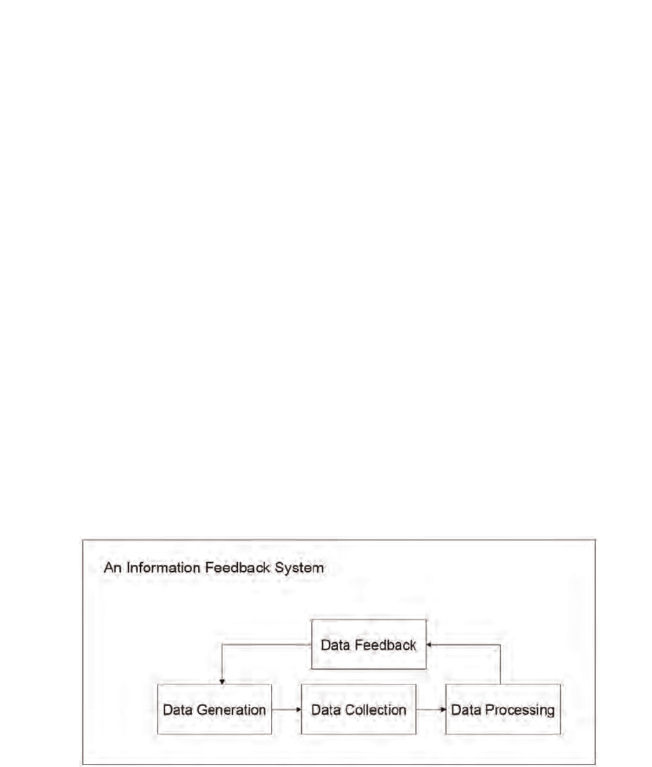
the existing infrastructure could be used more efficiently. Fig. 1 shows a schematic diagram
of an information feedback system, which demonstrates that feedback information plays a
significant role in the loop.
Fig. 1. The schematic diagram of an information feedback system.
Chuanfei Dong
1
and Binghong Wang
2,3
1
Georgia Institute of Technology
2
University of Science and Technology of China
3
University of Shanghai for Science and Technology and Shanghai Academy
of System Science
1
U.S.A.
2,3
P.R.China
Application of Cellular Automaton Model to
Advanced Information Feedback in Intelligent
Transportation Systems
11

Physics, other sciences and technologies meet at the frontier area of interdisciplinary research
(Helbing, 1996; Chowdhury et al., 2000; Helbing, 2001; Nagatani, 2002). The concepts and
techniques of physics are being applied to such complex systems as traffic systems. A
lot of theories have been proposed such as car-following theory (Rothery, 1992), kinetic
theory (Prigogine & Andrews, 1960; Paveri-Fontana, 1975; Helbing & Treiber, 1998) and
particle-hopping theory ( Nagel & Schreckenberg, 1992; Biham et al., 1992; Blue & Adler, 2001).
These theories provide insights that help traffic engineers and other professionals to better
manage congestion. Therefore these theories indirectly make contributions to alleviating
traffic congestion and enhancing the capacity of existing infrastructure. Although dynamics of
traffic flow with real-time traffic information have been extensively investigated (Friesz et al.,
1989; Arnott et al., 1991; Ben-Akiva et al., 1991; Mahmassani & Jayakrishnan, 1991; Kachroo
& Özbay, 1996; Yokoya, 2004), finding out a more efficient feedback strategy is still an overall
task. Recently, some information feedbacks have been proposed to investigate the two-route
scenario with the same length. Wahle et al. (2000 & 2002) firstly investigated the two-route
scenario with travel time feedback strategy (TTFS). Subsequently, Lee et al. (2001) studied the
effect of a different type of information feedback (MVFS), i.e. instantaneous average velocity.
Wang et al. (2005) proposed a third type of information feedback (CCFS), i.e. instantaneous
congestion coefficient which is defined as
C
=
q
∑
i=1
n
2
i
.(1)
where, n
i
stands for vehicle number of the ith congestion cluster in which cars are close to each
other without a gap between any two of them; q is the number of congestion clusters on the
route. Then Dong et al. (2010b) put forward another type of information feedback (WCCFS),
i.e. instantaneous weighted congestion coefficient which is defined as
C
w
=
p
∑
i=1
F(n
m
)n
2
i
.(2)
where the definition of n
i
is the same as above, F(n
m
) is the weight function, andn
m
stands for
the position of the ith congestion cluster. Here, we use the result of median rounding
n
m
of
the ith congestion cluster to represent its position. Furthermore, in order to provide road users
with better guidance, Dong et al. (2009a; 2009b; 2010a; 2010d) proposed another two types
of information feedback strategies named corresponding angle feedback strategy (CAFS)
and prediction feedback strategy (PFS), respectively. The corresponding angle coefficient is
defined as
C
θ
=
q
∑
i=1
θ
2
i
=
q
∑
i=1
arctan
(
n
first
i
H
) −arctan(
n
first
i
−l
i
H
)
2
.(3)
where n
first
i
stands for the position of the first vehicle in the ith congestion cluster, in which
vehicles are close to each other without a gap between any two of them. l
i
and θ
i
denote
the length and the weight (corresponding angle) of the ith congestion cluster, respectively.
H denotes the vertical distance from point T to the route (see Fig.2). In this chapter, we set
H
= 100. PFS is based on CCFS, and the predicted congestion coefficient (C
p
)isdefinedas:
C
p
(t)=C(t + Δt)=
q
∑
i=1
n
2
i
(t + Δt).(4)
238
Cellular Automata - Simplicity Behind Complexity
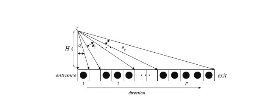
Fig. 2. Angles corresponding to different congestion clusters on the lane.
which indicates that PFS uses future road condition (the value of congestion coefficient C at
time t
+ Δt) as feedback information.
It has been proved that TTFS is the worst one which brings a lag effect to make it impossible
to provide the road users with the real situation of each route (Lee et al., 2001); CCFS is more
efficient than MVFS because the random brake mechanism of the Nagel-Schreckenberg (NS)
model (Nagel & Schreckenberg, 1992) brings fragile stability of velocity (Wang et al., 2005);
WCCFS i s more efficient than CCFS for the reason that CCFS does not take the weights of
different parts of the route into consideration (Dong et al., 2010b). However, WCCFS is still not
the best one due to the fact that the weight function F
(n
m
) does not contain any information
related to the length of the congestion cluster while the corresponding angle θ takes both
the length and route location of each cluster into account (Dong & Ma, 2010a). Though the
road capacity adopting PFS is the best one among these feedback strategies (Dong et al.,
2009a; Dong et al., 2009b; Dong et al., 2010d), the validity of PFS depends on the length of
the route when the traffic system is multi-route (Dong et al., 2010d). Also, PFS is not easy to
realize since it needs predicted road data, which will be discussed in detail in the following
paragraphs. We report the simulation results adopting six different feedback strategies TTFS,
MVFS, CCFS, WCCFS, CAFS and PFS in a two-route scenario with a single route following
the NS mechanism.
The chapter is arranged as follows: In Section 2, several cellular automaton models of traffic
flow will be mentioned including some analytical studies and a two-route scenario is briefly
introduced, together with s ix feedback strategies of TTFS, MVFS, CCFS, WCCFS, CAFS and
PFS all depicted in detail. In Section 3, some simulation results will be presented and discussed
based on the comparison of six different feedback strategies. In Section 4, we will make some
conclusions.
2. The model and feedback strategies
A. NS mechanism
Recently, a lot of cellular automaton models are proposed such as NS model (Nagel &
Schreckenberg, 1992), FI model (Fukui & Ishibashi, 1996), VDR model (Barlovic et al., 1998),
VE model (Li et al., 2001), BL model (Knospe et al., 2000), VE model (Li et al., 2001),
Kerner-Klenov-Wolf model (Kerner et al., 2002; Kerner & Klenov, 2004; Kerner, 2004), FMCD
model (Jiang & W u, 2003; Jiang & Wu, 2005), VDDR model (Hu et al., 2007), and VA model
(Gao et al., 2007). Also, a lot of analytical works based on statistical physics, such as the
239
Application of Cellular Automaton Model to
Advanced Information Feedback in Intelligent Transportation Systems

spacing-oriented mean field theory, have been studied to investigate fundamental diagrams
and asymptotic behavior of CA models, i.e., NS model, FI model, and NS & FI combined CA
model (Wang et al., 2000a; Wang et al., 2000b; Mao et al., 2003; Wang et al., 2003; Wang et
al., 2001; Fu et al., 2007). Among these CA models, the NS model is so far the most popular
and simplest cellular automaton model in analyzing the traffic flow (Nagel & Schreckenberg,
1992; Chowdhury et al., 2000; Helbing, 2001; Nagatani, 2002; Wang et al., 2002), where the
one-dimension CA with periodic boundary conditions is used to investigate highway and
urban traffic. This model can reproduce the basic features of real traffic like stop-and-go
wave, phantom jams, and the phase transition on a fundamental diagram that plots vehicle
flow versus density. Thus we still adopt NS model when comparing the effects of different
feedback strategies in this chapter. In the following paragraphs, the NS mechanism will be
briefly introduced as a basis of analysis.
The road is subdivided into cells (sites) with a length of Δx=7.5 m. The route length is set to
be L
= 2000 cells (corresponding to 15 km). N denotes the total number of vehicles on a single
route of length L. The vehicle density can be defined as ρ =N/L. A time step corresponds to
Δt
= 1s, the typical time a driver needs to react. g
n
(t) refers to the number of empty sites
in front of the nth vehicle at time t ,andv
n
(t) denotes the speed of the nth vehicle, i.e., the
number of sites that the nth vehicle moves during the time step t. In the present paper, we
set the maximum velocity v
max
= 3 cells/time step (corresponding to 81 km/h and thus a
reasonable value) for simplicity. The rules for updating the position x of a car are as follows. (i)
Acceleration: v
i
= min(v
i
+ 1, v
max
). (ii) Deceleration: v
i
= min(v
i
, g
i
) so as to avoid collisions,
where g
i
is the spacing in front of the ith vehicle. (iii) Random brake: with a certain probability
p that v
i
= max(v
i
−1, 0). (iv) Movement: x
i
= x
i
+ v
i
.
The fundamental diagram characterizes the basic properties of the NS model which has two
regimes called "free-flow" phase and "jammed" phase. The critical density, basically depending
on the random brake probability p, divides the fundamental diagram to these two phases.
The transition such as from "free-flow" phase to "jammed" phase is called transition on a
fundamental diagram (Nagel & Schreckenberg, 1992).
B. Two-route scenario
Recently, Wahle et al. (2000) investigated a two-route model. In their model, a percentage of
drivers (referred to as dynamic drivers) choose one of the two routes according to the real-time
information displayed on the roadside. In their model, the two routes A and B are of the same
length L. A new vehicle will be generated at the entrance of the traffic system at each time
step. If a driver is a so-called static one, he enters a route at random ignoring any advice.
The density of dynamic and static travelers are S
dyn
and 1 −S
dyn
, respectively. Once a vehicle
enters one of two routes, the motion of it will follow the dynamics of the NS model. In our
simulation, a vehicle will be removed after it reaches the end point. It is important to note
that if a vehicle cannot enter the preferred route, it will wait till the next time step rather than
entering the un-preferred route.
The simulations are performed by the following steps: first, we set the routes and boards
empty; second, let vehicles enter the routes randomly during the initial 100 time steps; third,
after the vehicles enter the routes, according to four different feedback strategies, information
will be generated, transmitted, and displayed on the board at each time step. Finally, the
dynamic road users will choose the route with better conditions according to the dynamic
information at the entrance of two routes.
C. Related definitions
240
Cellular Automata - Simplicity Behind Complexity
The road conditions can be characterized by the fluxes of two routes. The flux of the ith route
is defined as follows:
F
i
= V
i
mean
ρ
i
= V
i
mean
N
i
L
i
(5)
where L
i
represents the length of the ith route, V
i
mean
and N
i
denote the mean velocity of all
the vehicles and the vehicle number on the ith route, respectively. In this chapter, the physical
sense of flux F is the number of vehicles passing the exit of the traffic system each time step.
Therefore the larger the value of F, the better processing capacity the traffic system has.
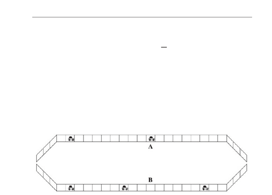
We assume the two-route system has only one entrance and one exit as shown in Fig.3. In
reality, there are different paths for drivers to choose from one place to another place. In this
chapter, we focus on a two-route system. Different drivers departing from the same place
could choose two different paths to get to the same destination which corresponds to the “one
entrance and one exit” system. Thus the road condition in present work is closer to reality
than some previous works (Wahle et al.,2000; Lee et al., 2001; Wang et al., 2005). The rules at
the exit of the two-route system are as follows:
Fig. 3. The one entrance and one exit two-route traffic system.
a) The special velocity update mechanism for the vehicle nearest to the exit:
i velocity(t)=Min(velocity(t)+1,3), (probability: 75%);
ii velocity(t)=Max(velocity(t)-1,0), (probability: 25%);
b) Rules at the exit when vehicles competing for driving out:
i At the end of two routes, the vehicle nearer to the exit goes first.
ii If the vehicles at the end of two routes have the same distance to the exit, the faster a
vehicle drives, the sooner it goes out.
iii If the vehicles at the end of two routes have the same speed and distance to the exit, the
vehicle in the route which has more vehicles drives out first.
iv If the rules (i), (ii) and (iii) are satisfied at the same time, then the vehicles go out
randomly.
c) velocity(t)=position(t)-position(t-1), where position(t)=L=2000; (valid only for the vehicles
failed in competing for driving out at exit);
Here we want to stress that the vehicle nearest to the exit will not obey the NS mechanism but
the special mechanism as shown in rule (a). However, vehicles following the vehicle closest
to the exit still obey the NS mechanism. One should also be aware that if the vehicle nearest
241
Application of Cellular Automaton Model to
Advanced Information Feedback in Intelligent Transportation Systems

to the exit does not compete with the vehicle on the other route for driving out or wins in the
competition, the vehicle will ignore rule (c). The special velocity update mechanism (rule (a))
is equivalent to the situation that 75% drivers exhibit aggressive behavior and 25% drivers
exhibit timid behavior near the exit, which is similar to the recent work studied by Laval &
Leclercq (2010). Please note that drivers exhibit timid behavior may also exhibit aggressive
behavior at next time step otherwise the timid drivers may stop at the exit all the time. Then
we describe six different feedback strategies as follows:
TTFS: The information of travel time on the board is set to be zero until one car leave the traffic
system. Each vehicle will be recorded the time when it enters and leaves one of the routes. We
use the difference between this two values as the feedback information. A new dynamic driver
will choose the road with shorter time shown on the information board.
MVFS: Every time step, the traffic control center will receive the velocity of each vehicle on the
route from GPS. They will deal with the information and display the mean velocity of vehicles
on each route on the information board. Road users at the entrance will choose one road with
larger mean velocity.
CCFS: Every time step, the traffic control center will receive the position of each vehicle on the
route from GPS. The work of the traffic control center is to compute the congestion coefficient
of each route and display it on the information board. Road users at the entrance will choose
one road with smaller congestion coefficient. The congestion coefficient is defined as
C
=
q
∑
i=1
n
w
i
.(6)
where n
i
stands for vehicle number of the ith congestion cluster in which cars are close to each
other without a gap between any two of them, and q denotes the total number of congestion
clusters on one route. Every cluster is evaluated by a weight w,wherew
= 2andonecan
check out that w
> 2 leads to the similar results with w = 2 (Wang et al., 2005).
WCCFS: Every time step, the traffic control center will receive data from the navigation system
(GPS) like CCFS, and the work of the center is to compute the congestion coefficient of each
road with a reasonable weighted function and display it on the information board. Road
users at the entrance will choose one road with smaller weighted congestion coefficient. The
weighted congestion coefficient is defined as Eq.(2).
After we try some functions such as F
(x)=cos(ax)+b and Gaussian function, we find
F
(x)=kx + b is the optimal one in terms of improving the capacity of the road. Here, we
set b
= 0 for the reason that it will cause the absolute weight value of the first route site
always to be the smallest when b
= 0. In this chapter, we set b = 2.0. Then we get the function
as follows:
F
(x)=k × x + b = k ×
n
m
2000
+ 2.0. (7)
Finally the expression of C
w
becomes
C
w
=
q
∑
i=1
F(n
m
)n
2
i
=
q
∑
i=1
(k ×
n
m
2000
+ 2.0) ×n
2
i
.(8)
We also find that how efficient the new strategy to improve the road capacity depends on the
value of the weight factor (slope - k) which we will discuss in detail in Section 3.
CAFS: Every time step, the traffic control center will receive data from the navigation system
(GPS) like CCFS. The work of the traffic control center is to compute the corresponding angle
242
Cellular Automata - Simplicity Behind Complexity

of each congestion cluster (see Fig.2) on the lane, sum square of each corresponding angle
up and display it on the information board. Road users at the entrance will choose one road
with smaller corresponding angle coefficient. The corresponding angle coefficient is defined
as Eq.(3).
PFS: Every time step, the traffic control center will receive data from the navigation system
(GPS) like CCFS. The work of the center is to compute the congestion coefficient of each route,
simulate the future road condition based on the current road condition by using CCFS, and
display the results on the information board. Road users at the entrance will choose one route
with smaller predicted congestion coefficient. For example, if the prediction time, T
p
,is50
seconds and the current time is the 100th second, the traffic control center will simulate the
road conditions in the next 50 seconds adopting CCFS, predict the road condition at the 150th
second, and show the result on the information board at the entrance of the route. Finally, road
users at the 100th second will choose one route with smaller predicted congestion coefficient at
the 150th second. By the same token, road users at the entrance at the 101th second will choose
one route with smaller predicted congestion coefficient at the 151th second like explained
above. The predicted congestion coefficient is defined as Eq.(4).
In the following section, performance by using six different feedback strategies will be shown
and discussed in detail.
3. Simulation results
Fig.4 (a) shows the dependence of average flux on weight factor ( k) by using WCCFS. As to
the routes’ processing capacity, we can see that in Fig.4 (a) there is a positive peak structure at
the vicinity of k
∼-1.98. Thus we will use k=-1.98 in the following paragraphs. Then Eq.(8) will
become C
w
=
∑
q
i
=1
(−1.98 ×
n
m
2000
+ 2.0) ×n
2
i
. In Fig.4 (b), we present the weight value of each
site on one route. One can find the weight value of the entrance is much larger than that of the
exit when using WCCFS and the reasons can be described as follows. First, in practice both
acceleration and deceleration shock waves travel at final velocities and – at least on average
– vehicles tend to be more affected by local traffic conditions than by conditions far ahead on
the roadway. This suggests that greater weight should be given to traffic conditions on the
upstream sections of each route. Second, the smaller weight value at the end of the route will
alleviate the negative effect of congestion caused by the traffic jam.
Since Fig.4 (a) shows the weight value of the entrance is larger than that of the exit when
adopting WCCFS, the point T located above the entrance of the route when adopting CAFS
(see Fig.2) is reasonable. It makes the weight of the entrance the largest. Furthermore, the
corresponding angle of each congestion cluster can reflect not only the weight of the route
but also the length of the congestion cluster. Therefore the weight value is more reasonable
than before (Dong et al., 2010a). Fig.4 (c) shows the dependence of average flux on position
of the pillar (point T) by using CAFS. As to the routes’ processing capacity, we can see that
the position of the pillar will directly affect the average flux. The average flux is much larger
when point T locates at the entrance of the route while the value is pretty lower when point
T locates at the end of the lane. Thus the result shown by Fig.4(c) is in accordance with that
indicated by Fig.4 (a). Also, this can be understood as shown in Fig.5, where the congestion
cluster on route A locates at the entrance of lane and the congestion cluster on route B locates
at the end of the lane. From Fig.5, we can see clearly that C
θ
of route A is larger than that of
route B, so the road user should enter route B instead of route A.IfpointT locate at the end of
the route, C
θ
of route A will smaller than that of route B, which will cause the vehicle to enter
route A. It will make the cluster larger or the vehicle even cannot enter the route.
243
Application of Cellular Automaton Model to
Advanced Information Feedback in Intelligent Transportation Systems
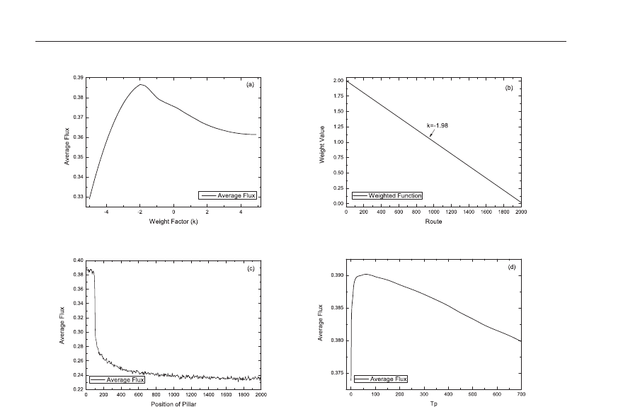
Fig. 4. (a) Average flux vs weight factor (k). The parameters are L=2000, p=0.25, and S
dyn
=0.5.
(b) Weight value of each site on one route. The parameters are L=2000, p=0.25, and S
dyn
=0.5.
(c) Average flux vs position of pillar (point T). The parameters are L=2000, p=0.25, S
dyn
=1.0
and vertical distance (H) is fixed to be 100. (d) Average flux vs prediction time (T
p
). The
parameters are L=2000, p=0.25, and S
dyn
=0.5.
Fig.4 (d) shows the dependence of average flux on prediction time (T
p
) by using PFS. As to
the routes’ processing capacity, we can see that in Fig.4 (d) there is a positive peak structure
at the vicinity of T
p
∼ 60. Thus we will use T
p
=60 in the following paragraphs. PFS is more
difficult to realize than other five feedback strategies since PFS is based on the future road
condition. As demonstrated by our previous work (Dong et al., 2010), more routes the traffic
system has, longer prediction time (T
p
) PFS needs (see Fig.6). The workload adopting CCFS
is equivalent to the workload adopting PFS when T
p
= 0 (which is equivalent to CCFS). Thus
in a two-route scenario, the workload of PFS is sixty times greater than that of CCFS because
the prediction time equal to 60 time steps (T
p
= 60). Given the time interval of every time
feedback is one time step, there is no doubt that PFS requires higher performance computers
to operate than the other five feedback strategies. It indicates that PFS will cost more to realize
than others.
Fig.7 shows simulation results of applying TTFS in a two-route scenario with respect to flux,
number of cars, and average speed all versus time step. The fluxes of two routes adopting
TTFS show oscillation (see Fig.7) obviously due to the information lag effect (Lee et al., 2001).
This lag effect can be understood. For TTFS, the travel time reported by a driver at the end of
two routes only represents the road condition in front of him, and perhaps the vehicles behind
him have got into the jammed state. Unfortunately, this information will induce more vehicles
244
Cellular Automata - Simplicity Behind Complexity
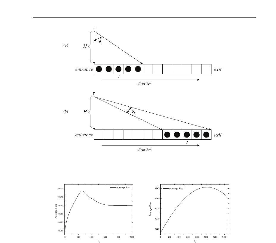
Fig. 5. The locations and corresponding angles of vehicle congestion clusters on route A and
route B.
Fig. 6. (a) Average flux vs prediction time (T
p
) in a three-route traffic system and T
p
(F
max
) ∼
260. (b) Average flux vs prediction time (T
p
) in a four-route traffic system and T
p
(F
max
) ∼
1020. The parameters are L=2000, p=0.25, and S
dyn
=0.5.
to choose his route until a vehicle from the jammed cluster leaves the system. This effect
apparently does harm to the system. Another reason for the oscillation is that the two-route
system only has one exit and the vehicle nearest to the exit obeys the special velocity update
mechanism; therefore at most one vehicle can go out each time step. It will result in the traffic
jam happening at the end of the route. Vehicle number versus time step shows almost the
same tendency as flux versus time step (see Fig.7 (b)) and the average velocity is around 2.4
cells per time step (refer to Fig.7(c)).
Fig.8 shows simulation results of applying MVFS in a two-route scenario with respect to flux,
vehicle number, and average speed all versus time step. The fluxes of two routes adopting
245
Application of Cellular Automaton Model to
Advanced Information Feedback in Intelligent Transportation Systems
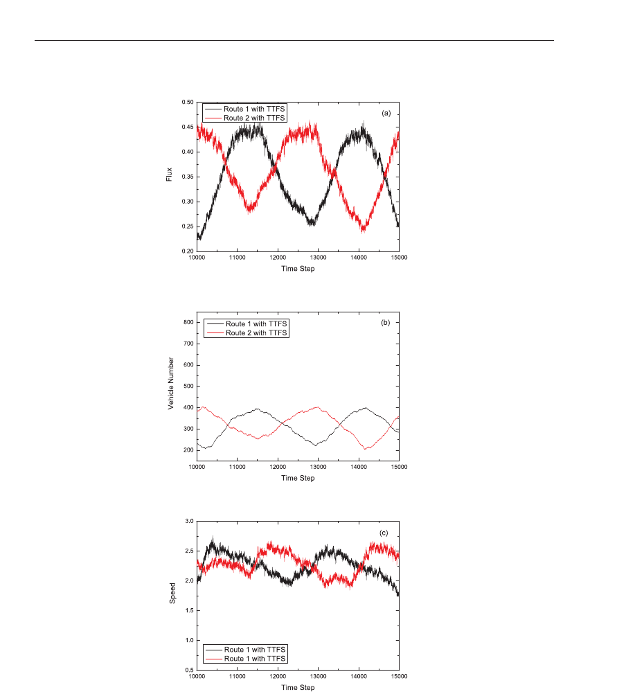
Fig. 7. (Color online)(a) Flux of each route with travel time feedback strategy. (b) Vehicle
number of each route with travel time feedback strategy. (c) Average speed of each route
with travel time feedback strategy. The parameters are L=2000, p=0.25 and S
dyn
=0.5.
246
Cellular Automata - Simplicity Behind Complexity