Samarskii A.A., Vabishchevich P.N. Numerical Methods for Solving Inverse Problems of Mathematical Physics

Подождите немного. Документ загружается.

86 Chapter 3 Boundary value problems for elliptic equations

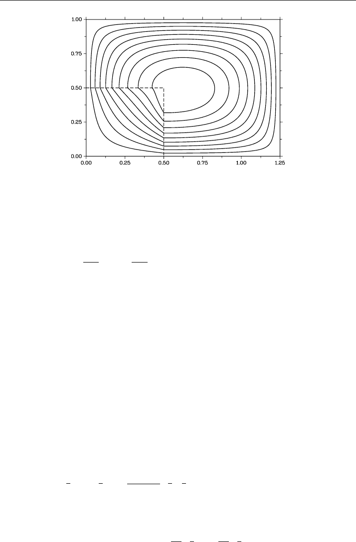
Figure 3.6 Solution obtained with κ

= 0.01

The calculation domain  in the method of ﬁctitious domains is dipped into the do-

main 

. Instead of the approximate solution of problem (3.64), (3.65), we deal with

the boundary value problem

−



α=1

∂

∂x



(x)

∂u

∂x



+ q

(x)u

= f

(x), x ∈ 

, (3.66)

(x) = 0, x ∈ ∂

. (3.67)

Consider a method of ﬁctitious domains with continuation over higher coefﬁcients in

which

(x), q

(x), f

(x) =



k(x), q(x), f (x), x ∈ ,

−2

, 0, 0, x ∈ 

= 

\.

Show that u

(x) − u(x)

()

→ 0asε → 0.

Exercise 3.2 Consider a method of ﬁctitious domains with continuation over lower

coefﬁcients for approximate solution of problem (3.64), (3.65), when in (3.66), (3.67)

we have:

(x), q

(x), f

(x) =



k(x), q(x), f (x), x ∈ ,

1,ε

−2

, 0, x ∈ 

= 

\.

Exercise 3.3 Show that the difference scheme

−y

− y

−

+ h

= ϕ(x), x ∈ ω,

y(x) = μ(x), x ∈ ∂ω

with

ϕ(x) = f (x) +

approximates the boundary value problem (3.2), (3.3) accurate to the fourth order.

Section 3.5 Exercises 87

Exercise 3.4 In the numerical solution of equation (3.1), approximate the third-kind

boundary condition

−k(0, x

)

∂u

∂x

+ σ(x

)u(0, x

) = μ(x

considered on one side of a rectangle  (on the other boundary segments, ﬁrst-kind

boundary conditions are given).

Exercise 3.5 Construct a difference scheme for the boundary value problem (3.1),

(3.3) with the following matched conditions at x

= x

∗

u(x

∗

+ 0, x

) − u(x

∗

− 0, x

) = 0,

∂u

∂x

∗

+ 0, x

) − k

∂u

∂x

∗

− 0, x

) = χ(x

Exercise 3.6 Consider the approximation of the second-order elliptic equation with

mixed derivatives

−



α,β=1

∂

∂x



αβ

(x)

∂u

∂x



= f (x), x ∈ ,

in which

αβ

(x) = k

βα

(x), α, β = 1, 2.

Exercise 3.7 In cylindrical coordinates, the Poisson equations in a circular cylinder

can be written as

−

∂

∂r



∂u

∂r



−

∂

∂ϕ

−

∂

∂z

= f (r,ϕ,z).

Construct a difference scheme for this equation with ﬁrst-kind boundary conditions on

the surface of the cylinder.

Exercise 3.8 Consider a difference scheme written as

A(x)y(x) −



ξ∈W



(x)

B(x,ξ)y(ξ ) = ϕ(x), x ∈ ω

with

A(x)>0, B(x,ξ)> 0,ξ∈ W



(x),

D(x) = A(x) −



ξ∈W



(x)

B(x,ξ)> 0, x ∈ ω.

Derive the following estimate for the solution of the problem:

y(x)

∞

≤



ϕ(x)

D(x)



∞

88 Chapter 3 Boundary value problems for elliptic equations

Exercise 3.9 Suppose that in the iteration method (of alternate directions)

k+1

− y

+ Ay

= ϕ, k = 0, 1,...

we have

A = A

+ A

, A

= A

and, in addition,

E ≤ A

≤ 

E, A

= A

∗

,δ

> 0,α= 1, 2.

Next, suppose that the operator B is given in the factorized form

B = (E + ν A

)(E + ν A

Find the optimum value of ν.

Exercise 3.10 To solve the difference problem

Ay = ϕ, A = A

∗

> 0

one uses the triangular iteration method

(D + τ A

)

k+1

− y

+ Ay

= ϕ,

with D being an arbitrary self-adjoint operator and

A = A

+ A

, A

= A

∗

Find the optimum value of τ if a priori information is given in the form

δ D ≤ A, A

−1

≤



Exercise 3.11 Derive the calculation formula

k+1

, r

)

(Aw

)

= B

−1

, r

= Ay

− ϕ

for the iteration parameter in the iterative steepest descend method

k+1

− y

k+1

+ Ay

= ϕ, k = 0, 1,...,

A = A

∗

> 0, B = B

∗

> 0,

from the condition of minimum norm of inaccuracy in H

at the next iteration.

Section 3.5 Exercises 89

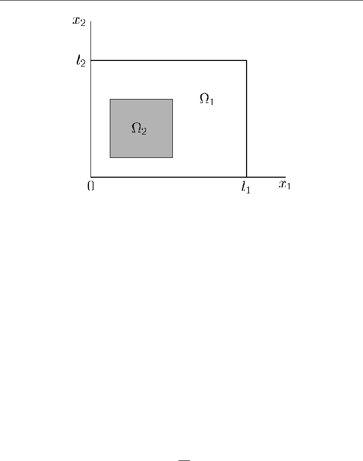
Figure 3.7 On the statement of the modiﬁed Dirichlet problem

Exercise 3.12 Using the program PROBLEM2, examine how the rate of convergence

in the used iterative process depends on the variable coefﬁcient k(x) (or, in the simplest

case, how the number of iterations depends on κ

Exercise 3.13 Using the program PROBLEM2, perform numerical experiments on

solving the Dirichlet problem in a step domain 

(Figure 3.3) based on the method

of ﬁctitious domains with continuation over lower coefﬁcients.

Exercise 3.14 Modify the program PROBLEM2 so that to solve the third boundary

value problem (boundary conditions (3.4)) for equation (3.60).

Exercise 3.15 Consider the modiﬁed Dirichlet problem for equation (3.1) in a bicon-

nected domain 

(Figure 3.7). At the outer boundary, conditions (3.1) are given. At

the internal boundary, the solution is constant, but this solution itself must be deter-

mined from an additional integral condition:

u(x) = const, x ∈ ∂



∂

k(x)

∂u

∂n

dx = 0.

To approximately solve the problem, use the method of ﬁctitious domains imple-

mented via the program PROBLEM2.

4 Boundary value problems

for parabolic equations

As a typical non-stationary mathematical physiscs problem, we consider here the

boundary value problem for the space-uniform second-order equation. On the approx-

imation over space, we arrive at a Cauchy problem for a system of ordinary differential

equations. Normally, the approximation over time in such problems can be achieved

using two time layers. Less frequently, three-layer difference schemes are used. A

theoretical consideration of the convergence of difference schemes for non-stationary

problems rests on the theory of stability (correctness) of operator-difference schemes

in Hilbert spaces of mesh functions. Conditions for stability of two- and three-layer

difference schemes under various conditions are formulated. Numerical experiments

on the approximate solution of a model boundary value problem for a one-dimensional

parabolic equation are performed.

4.1 Difference schemes

Difference schemes for a model second-order parabolic equation are constructed. The

approximation over time is performed using two and three time layers.

4.1.1 Boundary value problems

Consider a simplest boundary value problem for a one-dimensional parabolic equation.

The calculation domain is the rectangle

=  × [0, T ],  ={x | 0 ≤ x ≤ l}, 0 ≤ t ≤ T .

The solution is to be found from the equation

∂u

∂t

∂

∂x



k(x)

∂u

∂x



+ f (x, t), 0 < x < l, 0 < t ≤ T. (4.1)

Here, the coefﬁcient k depends just on the spatial variable and, in addition, k(x) ≥

κ>0.

We consider the ﬁrst boundary value problem (with the boundary conditions as-

sumed homogeneous) in which equation (4.1) is supplemented with the conditions

u(0, t) = 0, u(l, t) = 0, 0 < t ≤ T. (4.2)

Also, the following initial conditions are considered:

u(x, 0) = u

(x), 0 ≤ x ≤ l. (4.3)

Section 4.1 Difference schemes 91

In a more general case, one has to use third-kind boundary conditions. In the latter

case, instead of (4.2) we have:

−k(0)

(0, t) + σ

(t)u(0, t) = μ

(t),

k(l)

(l, t) + σ

(t)u(l, t) = μ

(t), 0 < t ≤ T.

(4.4)

The boundary value problem (4.1)–(4.3) is considered as a Cauchy problem for the

ﬁrst-order differential-operator equation in the Hilbert space H = L

() for functions

deﬁned in the domain  = (0, 1) and vanishing at the boundary points of the domain

(on ∂). For the norm and for the scalar product, we use the settings

(v, w) =



v(x)w(x) dx, v

= (v, v) =



(x) dx.

We deﬁne the operator

Au =−

∂

∂x



k(x)

∂u

∂x



, 0 < x < l, (4.5)

for functions satisfying the boundary conditions (4.2).

The boundary value problem (4.1)–(4.3) is written as a problem in which it is re-

quired to ﬁnd the function u(t) ∈ H from the differential-operator equation

+ Au = f (t), 0 < t ≤ T (4.6)

supplemented with the initial condition

u(0) = u

. (4.7)

The operator A is a self-adjoint operator positively deﬁned in H, i. e.,

∗

= A ≥ mE, m = κπ

> 0. (4.8)

With the aforesaid taken into account (see the proof of Theorem 1.2), we derive the

following a priori estimate for the solution of problem (4.6)–(4.8):

u(t)≤exp (−mt )



u

+



exp (mθ) f (θ)dθ



. (4.9)

A cruder estimate derived by invoking the property of non-negativeness of the op-

erator A only was obtained previously in Theorem 1.2; this estimate has the form

u(t)≤u

+



 f (θ )dθ. (4.10)

Estimates (4.9) and (4.10) show that the solution of problem (4.6)–(4.8) is stable

with respect to initial data and right-hand side. Such fundamental properties of the

differential problem must be inherited when we pass to a discrete problem.

92 Chapter 4 Boundary value problems for parabolic equations

4.1.2 Approximation over space

As usually, we denote as ¯ω a uniform grid with stepsize h over the interval

 = [0, l]:

¯ω ={x | x = x

= ih, i = 0, 1,...,N, Nh = l}

and let ω and ∂ω be the sets of internal and boundary nodes.

At internal nodes, we approximate the differential operator (4.5), accurate to the

second order, with the difference operator

Ay =−(ay

¯x

)

, x ∈ ω, (4.11)

in which, for instance, a(x) = k(x − 0.5h).

In the mesh Hilbert space H , we introduce a norm deﬁned as y=(y, y)

1/2

where

(y,w) =



x∈ω

y(x)w(x)h.

On the set of functions vanishing on ∂ω, for the self-adjoint operator A under the

constraints k(x) ≥ κ>0 and q(x) ≥ 0 there holds the estimate

A = A

∗

≥ κλ

E, (4.12)

in which

sin

πh

≥

is the minimum eigenvalue of the difference operator of second derivative on the uni-

form grid.

The approximation over space performed, we have the following problem put into

correspondence to the problem (4.6), (4.7):

+ Ay = f, x ∈ ω, t > 0, (4.13)

y(x, 0) = u

(x), x ∈ ω. (4.14)

By virtue of (4.12), for the solution of problem (4.13), (4.14) there holds the esti-

mate

y(x, t)≤exp (−κλ



u

(x)+



exp (κλ

θ) f (x,θ)dθ



, (4.15)

consistent with estimate (4.9).

Section 4.1 Difference schemes 93

4.1.3 Approximation over time

The next step in the approximate solution of the Cauchy problem for the system of

ordinary difference equations (4.13), (4.14) is approximation over time. We deﬁne a

time-uniform grid

¯ω

= ω

∪{T }={t

= nτ, n = 0, 1,...,N

,τN

= T }.

We denote as A, B : H → H linear operators in H dependent, generally speaking,

on τ and t

. In the notation used below, following the manner adopted in the theory of

difference schemes, we do not use subscripts:

y = y

, ˆy = y

n+1

, ˇy = y

n−1

y −ˇy

, y

ˆy − y

In a two-layer difference scheme used to solve a non-stationary equation, the transi-

tion to the next time layer t = t

n+1

is performed using the solution y

at the previous

time layer.

In the two-layer scheme, equation (4.13) is approximated with the difference equa-

tion

n+1

− y

+ A(σ y

n+1

+ (1 − σ)y

) = ϕ

, n = 0, 1,...,N

− 1, (4.16)

where σ is a numerical parameter (weight) to be taken from the interval 0 ≤ σ ≤ 1.

For the right-hand side, one can put, for instance,

= σ f

n+1

+ (1 − σ)f

Approximation of (4.14) yields

= u

(x), x ∈ ω. (4.17)

Scheme (4.16) is known as the weighted scheme.

For the time-approximation inaccuracy of the ﬁrst derivative we have:

n+1

− v

∗

) + O(τ

where ν = 2ift = t

n+1/2

; otherwise, ν = 1. As a result, we obtain the difference

equation (4.16) that approximates equation (4.13) over time accurate to the second

order in the case of σ = 0.5 and accurate to the ﬁrst order in the case of σ = 0.5.

Consider also the weighted three-layer difference scheme for equation (4.13), in

which three time layers (t

n+1

, t

and t

n−1

) are used:



n+1

− y

+ (1 − θ)

− y

n−1



+ A(σ

n+1

+ (1 − σ

− σ

+ σ

n−1

) = ϕ

, (4.18)

94 Chapter 4 Boundary value problems for parabolic equations

n = 1, 2,...,N

− 1.

For the right-hand side, it would appear reasonable to use the approximations

= σ

n+1

+ (1 − σ

− σ

) f

+ σ

n−1

Now, we can enter the three-layer calculation scheme with known y

and y

= u

, y

= u

. (4.19)

For y

, we use the initial condition (4.14). To ﬁnd y

, we invoke a two-layer difference

scheme, for instance,

− y

A(y

+ y

) =

( f

+ f

The difference scheme (4.18), (4.19) involves a weighting parameter θ used in the ap-

proximation of the time derivative and two weighting parameters, σ

and σ

, used in

the approximation of other terms. Let us give some typical sets of weighting parame-

ters that have found use in practical computations.

Using a greater number of layers in approximation of time-dependent equations is

aimed, ﬁrst of all, at raising the approximation order. That is why in the considera-

tion of three-layer schemes (4.18), (4.19) it makes sense for us to restrict ourselves to

schemes that approximate the initial problem (4.13), (4.14) over time with an order not

less than second order.

First of all, consider a one-parametric family of symmetric schemes of the second

approximation order

n+1

− y

n−1

2τ

+ A(σ y

n+1

+ (1 − 2σ)y

+ σ y

n−1

) = ϕ

, (4.20)

which results from (4.18) with the settings

θ = 1/2,σ= σ

= σ

Particular attention should be paid to the scheme

n+1

− 4y

+ y

n−1

2τ

+ Ay

n+1

= ϕ

(4.21)

that approximates equation (4.13) accurate to O(τ

) with properly given right-hand

side (for instance, ϕ

= f

n+1

). Note that if in (4.18) we choose

θ = 3/2,σ

= 1,σ

= 0,

then we arrive at scheme (4.21).

Section 4.2 Stability of two-layer difference schemes 95

4.2 Stability of two-layer difference schemes

A highly important place in the robustness study of approximate solution methods for

non-stationary problems is occupied by the stability theory. Below, we introduce key

notions in use in the theory of stability for operator-difference schemes considered in

ﬁnite-dimensional Hilbert spaces, formulate stability criteria for two-layer difference

schemes with respect to initial data, and give typical estimates of stability with respect

to initial data and right-hand side.

4.2.1 Basic notions

Stability conditions are formulated for difference schemes written in the uniﬁed gen-

eral (canonical) form. Any two-layer scheme can be written in the form

B(t

)

n+1

− y

+ A(t

= ϕ

, t

∈ ω

, (4.22)

= u

, (4.23)

where y

= y(t

) ∈ H is the function to be found and the functions ϕ

, u

∈ H

are given functions. Notation (4.22), (4.23) is called the canonical form of two-layer

schemes.

For the Cauchy problem at the next time layer to be solvable, we assume that the

operator B

−1

does exist. Then, we can write equation (4.22) as

n+1

= Sy

+ τ ˜ϕ

, S = E − τ B

−1

A, ˜ϕ

= B

−1

. (4.24)

The operator S is called the transition operator for the two-layer difference scheme

(using this operator, transitions from one time layer to the next time layer can be per-

formed).

A two-layer scheme is called stable, if there exist positive constants m

and m

independent of τ and, also, of u

and ϕ, such that for all u

∈ H, ϕ ∈ H, and t ∈¯ω

for the solution of problem (4.22), (4.23) the following estimate is valid:

y

n+1

≤m

u

+m

max

0≤θ≤t

ϕ(θ)

∗

, t

∈ ω

. (4.25)

Here ·and ·

∗

are some norms in the space H . Inequality (4.25) implies that the

solution of problem (4.22), (4.23) depends continuously on input data.

The difference scheme

B(t

)

n+1

− y

+ A(t

= 0, t

∈ ω

, (4.26)

= u

(4.27)

is called a scheme stable with respect to initial data, if for the solution of problem

(4.26), (4.27) the following estimate holds:

y

n+1

≤m

u

, t

∈ ω

. (4.28)