Samarskii A.A., Vabishchevich P.N. Numerical Methods for Solving Inverse Problems of Mathematical Physics

Подождите немного. Документ загружается.

196 Chapter 6 Right-hand side identiﬁcation

DIMENSION VT(M), VY(M), VP(M), VV(M)

+ ,A(N), B(N), C(N), F(N), Y(N), VB(N), FB(N), W(N), Z(N)

C PARAMETERS:

C XL, XR - LEFT AND RIGHT END POINTS OF THE SEGMENT;

C XD - OBSERVATION POINT;

C N - NUMBER OF GRID NODES OVER THE SPATIAL VARIABLE;

C TMAX - MAXIMAL TIME;

C M - NUMBER OF GRID NODES OVER TIME;

C DELTA - INPUT-DATA INACCURACY;

C VY(M) - EXACT SOLUTION AT THE OBSERVATION POINT;

C VP(M) - DISTURBED SOLUTION AT THE OBSERVATION POINT;

C VT(M) - EXACT TIME DEPENDENCE OF THE RIGHT-HAND SIDE;

C VB(N)) - DEPENDENCE OF THE RIGHT-HAND SIDE ON THE SPATIAL

C VARIABLE;

C VV(M) - CALCULATED RIGHT-HAND SIDE VERSUS TIME;

XL = 0.D0

XR = 1.D0

XD = 0.3D0

TMAX = 1.D0

OPEN (01, FILE = ’RESULT.DAT’) ! FILE TO STORE THE CALCULATED DATA

C GRID

H=(XR-XL)/(N-1)

TAU = TMAX / (M-1)

ND = 1 + (XD + 0.5D0

H)/H

C DIRECT PROBLEM

C SOURCE

DOK=1,M

T = (K-0.5D0)

TAU

VT(K) = (K-0.5D0)

TAU

IF (T.GE.0.6D0) VT(K) = 0.D0

END DO

C DEPENDENCE OF THE RIGHT-HAND SIDE ON THE SPATIAL VARIABLE

DOI=1,N

VB(I) = DSIN(3.1415926

(I-1)

END DO

C SOLUTION OF THE PROBLEM

C INITIAL CONDITION

T = 0.D0

DOI=1,N

Y(I) = 0.D0

END DO

VY(1) = Y(ND)

Section 6.3 Reconstruction of the time-dependent right-hand side 197

C NEXT TIME LAYER

DOK=2,M

T=T+TAU

C DIFFERENCE-SCHEME COEFFICIENTS

DOI=2,N-1

A(I) = 1.D0 / (H

B(I) = 1.D0 / (H

C(I) = 2.D0 / (H

H) + 1.D0 / TAU

END DO

C BOUNDARY CONDITIONS AT THE LEFT AND RIGHT END POINTS

B(1) = 0.D0

C(1) = 1.D0

F(1) = 0.D0

A(N) = 0.D0

C(N) = 1.D0

F(N) = 0.D0

C RIGHT-HAND SIDE OF THE DIFFERENCE EQUATION

DOI=2,N-1

F(I) = VB(I)

VT(K) + Y(I) / TAU

END DO

C SOLUTION AT THE NEXT TIME LAYER

ITASK = 1

CALL PROG3 ( N, A, C, B, F, Y, ITASK )

VY(K) = Y(ND)

END DO

C DISTURBING OF MEASURED QUANTITIES

DO K = 1,M

VP(K) = VY(K) + 2.D0

DELTA

(RAND(0)-0.5D0)

END DO

C INVERSE PROBLEM

C AUXILIARY FUNCTION

DOI=2,N-1

FB(I) = ( 1.D0 / VB(ND) )

(VB(I+1)-2.D0

VB(I) + VB(I-1)) / (H

END DO

C SOLUTION OF THE PROBLEM

C INITIAL CONDITION

T = 0.D0

DOI=1,N

Y(I) = 0.D0

END DO

198 Chapter 6 Right-hand side identiﬁcation

C NEXT TIME LAYER

DOK=2,M

T=T+TAU

C DIFFERENCE-SCHEME COEFFICIENTS

DOI=2,N-1

A(I) = 1.D0 / (H

B(I) = 1.D0 / (H

C(I) = 2.D0 / (H

H) + 1.D0 / TAU

END DO

C BOUNDARY CONDITIONS AT THE LEFT AND RIGHT END POINTS

B(1) = 0.D0

C(1) = 1.D0

F(1) = 0.D0

A(N) = 0.D0

C(N) = 1.D0

F(N) = 0.D0

C RIGHT-HAND SIDE OF THE DIFFERENCE EQUATION

DOI=2,N-1

F(I) = FB(I)

VY(K) + Y(I) / TAU

END DO

C SOLUTION OF THE FIRST SUBPROBLEM AT THE NEXT TIME LAYER

ITASK = 1

CALL PROG3 ( N, A, C, B, F, W, ITASK )

C DIFFERENCE-SCHEME COEFFICIENTS

DOI=2,N-1

A(I) = 1.D0 / (H

B(I) = 1.D0 / (H

C(I) = 2.D0 / (H

H) + 1.D0 / TAU

END DO

C BOUNDARY CONDITIONS AT THE LEFT AND RIGHT END POINTS

B(1) = 0.D0

C(1) = 1.D0

F(1) = 0.D0

A(N) = 0.D0

C(N) = 1.D0

F(N) = 0.D0

C RIGHT-HAND SIDE OF THE DIFFERENCE EQUATION

DOI=2,N-1

F(I) = - FB(I)

END DO

Section 6.3 Reconstruction of the time-dependent right-hand side 199

C SOLUTION OF THE SECOND SUBPROBLEM AT THE NEXT TIME LAYER

ITASK = 1

CALL PROG3 ( N, A, C, B, F, Z, ITASK )

VV(K) = (VP(K)-VP(K-1)

+ - (W(ND) / (1 - Z(ND)) - Y(ND) )) / (TAU

VB(ND))

DOI=1,N

Y(I) = W(I) + Z(I)

W(ND) / (1 - Z(ND))

END DO

C APPROXIMATE SOLUTION

WRITE ( 01,

) (VV(K), K = 2,M)

WRITE ( 01,

) (VT(K), K = 2,M)

CLOSE (01)

STOP

END

6.3.5 Computational experiments

Below, results of calculations are presented which were carried out for the simplest

model inverse problem (6.84)–(6.89). Within the concept of quasi-real experiment, we

consider the direct problem (6.84)–(6.87) with some given right-hand side. For the

equation coefﬁcient and for the initial condition we put:

k(x) = 1, u

(x) = 0, 0 ≤ x ≤ 1.

The right-hand side is deﬁned as

ψ(x) = sin (π x), 0 ≤ x ≤ 1,

η(t) =



t, 0 < t < 0.6,

0, 0.6 < t < T = 1.

This problem was solved numerically on a grid with N = 100, N

= 100.

Below, we give data obtained by reconstructing the right-hand side from observa-

tions performed at the point x

∗

= 0.3. The calculated data were used to specify the

mesh function ϕ

In the solution of the inverse problem, the mesh function ϕ(t) was perturbed using

random inaccuracies. We put

= ϕ

+ 2δ(σ

− 1/2),

where σ

is a random function normally distributed over the interval [0, 1]. The quan-

tity δ deﬁnes the inaccuracy level. Figure 6.9 presents, as a function of time, the exact

right-hand side and the right-hand side reconstructed by the above algorithm at the

inaccuracy level δ = 0.001.

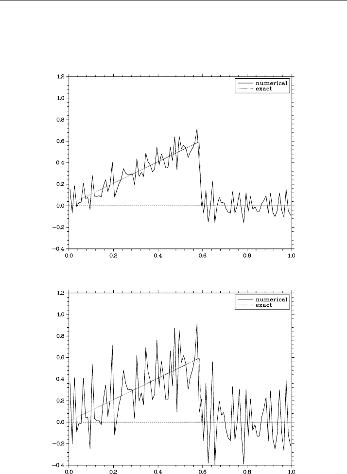
200 Chapter 6 Right-hand side identiﬁcation

Figure 6.9 Reconstructed right-hand side versus time at δ = 0.001

Figure 6.10 Solution of the inverse problem obtained with δ = 0.0025

Section 6.4 Identiﬁcation of time-independent right-hand side: parabolic equations 201

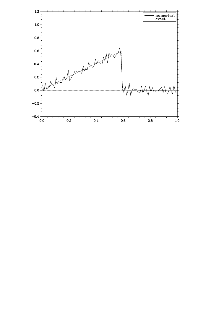
Figure 6.11 Solution of the inverse problem obtained with δ = 0.0005

Correctness of the considered inverse problem is illustrated by calculation data ob-

tained at various inaccuracy levels. Figures 6.10 and 6.11 show the solutions of the

problem obtained with δ = 0.0025 and δ = 0.0005, respectively. The lower is the

inaccuracy level, the more accurately can the solution be reconstructed.

The considered computational algorithm for solving the inverse problem can be used

to solve more general problems. In particular, multi-dimensional problems, problems

with many observation points, etc. can be treated much in the same manner. Fun-

damental difﬁculties (ill-posedness) arise when we pass to problems with localized

sources, with abandoned assumption ψ(x

∗

) = 0.

6.4 Identiﬁcation of a time-independent

right-hand side of a parabolic equation

Below, we consider an inverse problem in which it is required to reconstruct the time-

independent right-hand side of a parabolic equation. Additional measurements are

assumed to be performed at the end time.

6.4.1 Statement of the problem

Consider a process governed by a second-order one-dimensional parabolic equation.

We assume that the dynamics of interest is deﬁned by a time-independent, spatially

distributed source, so that

∂u

∂t

∂

∂x



k(x)

∂u

∂x



+ f (x), 0 < x < l, 0 < t ≤ T. (6.110)

202 Chapter 6 Right-hand side identiﬁcation

We supplement this equation with ﬁrst-kind homogeneous boundary conditions:

u(0, t) = 0, u(l, t) = 0, 0 ≤ t ≤ T. (6.111)

The initial state is deﬁned by the condition

u(x, 0) = 0, 0 < x < l. (6.112)

With given coefﬁcient k(x) and right-hand side f (x), relations (6.110)–(6.112) deﬁne

the direct problem.

Consider an inverse problem in which the unknown quantity is the right-hand side

f (x) of equation (6.110). We assume that the function f (x) can be reconstructed from

the known end-time solution; i.e., this function can be represented as

u(x, T ) = ϕ(x), 0 < x < l. (6.113)

To begin with, obtain an a priori estimate for the solution u(x, t) of the problem that

proves the solution to be stable with respect to weak perturbations of ϕ(x).

6.4.2 Estimate of stability

The simplest approach to the inverse problem (6.110)–(6.113) consists in elimination

of the unknown function ϕ(x). To this end, we differentiate the equation (6.110) with

respect to time:

∂

∂t

∂

∂x



k(x)

∂

∂x∂t



, 0 < x < l, 0 < t < T. (6.114)

For the latter equation, two boundary conditions, (6.112) and (6.113), are given for the

variable t.

For the problem (6.111)–(6.114), we use the operator notation that can be used to

study more general problems. We introduce a Hilbert space L

() with the following

scalar product and norm:

(v, w) =



v(x)w(x) dx, v

= (v, v) =



(x) dx.

For the functions v(x, t), w(x, t) from H = L

),weput

(v, w)

∗



(v, w) dt =



v(x)w(x) dx dt, v

∗

= ((v, v)

∗

)

1/2

On the set of functions satisfying the conditions (6.111), we deﬁne the operator

Au =−



k(x)



Section 6.4 Identiﬁcation of time-independent right-hand side: parabolic equations 203

Among of the main properties of A in L

(), the following property deserves mention:

A = A

∗

≥ mE, m > 0.

Using the settings introduced, reformulate the problem (6.111)–(6.114) as the fol-

lowing boundary value problem:

+ A

= 0, 0 < t < T, (6.115)

u(0) = 0, u(T ) = ϕ. (6.116)

We pass from (6.115), (6.116) to a problem with homogeneous boundary conditions.

To do so, we represent the solution as

u(t) = w(t) +

ϕ. (6.117)

For the function w(t), we obtain the problem

+ A

=−ψ, 0 < t < T , (6.118)

w(0) = 0,w(T ) = 0, (6.119)

where

ψ =

Aϕ.

To derive a simplest a priori estimate for the solution of problem (6.118), (6.119),

we scalarwise multiply equation (6.118) in H by w:





∗





∗

=−(ψ, w)

∗

. (6.120)

Consideration of the constancy of A and the homogeneous boundary conditions

(6.119) gives





∗



(Aw, w) =

(Aw, w)



= 0.

With (6.119) taken into account, for the ﬁrst term in (6.120) we obtain





∗

=−





=−









dt, 1



Then, substitution into (6.20) yields:









dt, 1



= (ψ, w)

∗

. (6.121)

204 Chapter 6 Right-hand side identiﬁcation

The left-hand side of (6.121) can be estimated by invoking the Friedrichs inequality



dt ≤ M







dt.

By virtue of this, we have









dt, 1



≥ M

−1

(w

∗

)

For the right-hand side of (6.121), we use the estimate

(ψ, w)

∗

≤ψ

∗

w

∗

This allows us to obtain from (6.121) the desired inequality

w

∗

≤ M

ψ

∗

, (6.122)

which shows that the solution of problem (6.118), (6.119) is stable with respect to the

right-hand side.

With allowance for (6.122) and (6.117), for the solution of problem (6.115), (6.116)

we obtain

u

∗

≤ϕ

∗

Aϕ

∗

. (6.123)

Thus, in the inverse problem (6.115), (6.116) the solution u(t) continuously depends

on the conditions at t = T .

With the function u(t) found from the solution of the well-posed problem (6.115),

(6.116), the sought right-hand side f is given by

f =

+ Au. (6.124)

A complete study of well-posedness of the inverse problem for the pair of functions

{u, f } poses the question how the functions u and f depend on the input data (on the

function ϕ). Above, we have restricted ourselves to obtaining the simplest estimate

(6.123) only for u.

6.4.3 Difference problem

The difference problem (6.110)–(6.113) reduces to the non-classical boundary value

problem (6.111)–(6.114). It makes sense to consider speciﬁc features of the computa-

tional algorithm, with special emphasis placed to the matter of time discretization. For

the mesh functions we use the same notation as for the continuous-argument functions.

For spatial discretization, we use a uniform grid ¯ω with a grid size h over the interval

 = [0, l]:

¯ω ={x | x = x

= ih, i = 0, 1,...,N, Nh = l},

Section 6.4 Identiﬁcation of time-independent right-hand side: parabolic equations 205

where, as usual, ω is the set of internal nodes and ∂ω is the set of boundary nodes. In

the mesh Hilbert space L

(ω), we introduce the norm via the relation y=(y, y)

1/2

where

(y,w) =



x∈ω

y(x)w(x)h.

At internal nodes, we approximate the differential operator A with second order,

with the difference operator

Ay =−(ay

¯x

)

, x ∈ ω, (6.125)

where, for instance, a(x) = k(x − 0.5h).

On the set of functions vanishing on ∂ω (see (6.111)) for the self-adjoint operator A

under the constraints k(x) ≥ κ>0 and q(x) ≥ 0 there holds the estimate

A = A

∗

≥ κλ

E (6.126)

with a constant

sin

πh

≥

Over time, we use the uniform grid

¯ω

= ω

∪{T }={t

= nτ, n = 0, 1,...,N

,τN

= T }

and let y

= y(t

To approximate equation (6.114) with second order over time and space, we can

naturally use the difference equation

n+1

− 2u

+ u

n−1

+ A

n+1

− u

n−1

2τ

= 0,

x ∈ ω, n = 1, 2,...,N

− 1.

(6.127)

This equation is supplemented with the boundary conditions (see (6.112), (6.113))

= 0, u

= ϕ, x ∈ ω. (6.128)

The difference problem (6.127), (6.128) can be examined analogously to the differ-

ential case. We represent (see (6.117)) the difference solution as

= w

ϕ, n = 0, 1,...,N

. (6.129)

The analogue of (6.118), (6.119) is the problem

n+1

− 2w

+ w

n−1

+ A

n+1

− w

n−1

2τ

=−ψ,

x ∈ ω, n = 1, 2,...,N

− 1,

(6.130)