Sandau R. Digital Airborne Camera: Introduction and Technology

Подождите немного. Документ загружается.

2.5 Sampling 71

Comparing (2.5-3) and (2.5-4), it can be seen that the Fourier coefﬁcients a

are

proportional to the sampling values f(t

) of the signal f(t):

2ν



2ν



. (2.5-5)

If one chooses the sampling points according to

= n ·t =

2ν

, (2.5-6)

then, since ν

> ν

, the distance t of sampling points must be smaller than

t

max

2ν

. (2.5-7)

in order not to lose information.

If the condition t < t

max

is fulﬁlled and the sampling values f(n·t) are given,

then the spectrum F(ν) may be calculated according to (2.5-2) and (2.5-5). The

same must also be true for the function f(t), because it is uniquely determined by

F(ν). From (2.5-2), (2.5-4) and (2.5-5), Shannon’s sampling theorem

(

)

+∞



n=−∞



2ν



sin



2πν



t −

2ν



2πν



t −

2ν



(2.5-8)

(

)

+∞



n=−∞

(

nt

)

sin



t

(

t −nt

)



t

(

t −nt

)

; t =

2ν

. (2.5-8a)

is obtained.

The sampling theorem (2.5-8) allows the calculation of any value of f(t)ifall

sampled values f(n·t) are given. Of course, in reality only a ﬁnite number of sam-

pling values is available (e.g. f(n·t)for–N ≤ n ≤ N), resulting in an error which

can be estimated if one has some knowledge about f(t)for|t|→∞.

A different kind of errors arises if the sampling distance t is chosen greater

than t

max

(or ν

< ν

), called undersampling. Incorrect contributions at some fre-

quencies inside –ν

< ν < ν

may occur which can substantially distort the function

f(t) (which is calculated from the sampling values using the sampling theorem or

another interpolation formula).

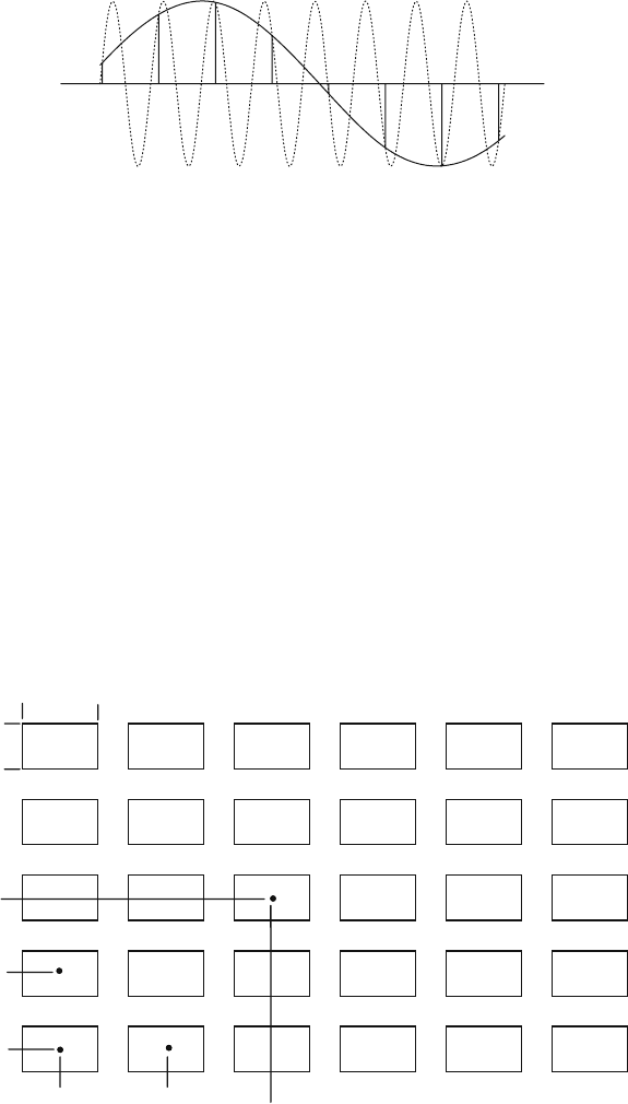
This behaviour can be demonstrated using the function sin(2πν

t) (see

Fig. 2.5-1): the dotted curve in Fig. 2.5-1 is the function sin(2πν

t) and the vertical

bars are the sampling values. There is strong undersampling because the sampling

distance is bigger than a whole period of the sine-function (less than half a period

is allowed). Interpolation of the sampling values using Shannon’s sampling theo-

rem leads to a function which is presented as the solid curve in Fig. 2.5-1. This

72 2 Foundations and Deﬁnitions

Fig. 2.5-1 Undersampling

is also a sine-function but with incorrect (too low) frequency. In sampled images

(see Fig. 2.5-4), this effect may be seen impressively because the eye interpolates

between the sampling points (picture elements, pixels).

Optoelectronic sensors sample images too. The problems that arise will be dis-

cussed now. It was shown in Section 2.4 that an optical system has band-limiting

properties because of diffraction (see (2.4-25) and Fig. 2.4-9). Spatial frequencies

k > k

of the scene will be cut off and do not occur in the image, which means

that the scene is smoothed. If one samples images using optoelectronic sensors (e.g.

CCD or CMOS sensors), this should be taken into account, especially when there

are periodic structures in the scene that cause aliasing.

The optoelectronic detectors used today are assembled by detector elements

arranged in a periodic way. Figure 2.5-2 shows (idealized) rectangular detector ele-

ments with central points (x

) and linear dimensions δ

, δ

. The detector elements

have the pitch 

and 

with 

≥δ

und 

≥δ

. I f the detector array according

δy

δx

Δy

Δx

Fig. 2.5-2 Detector array

2.5 Sampling 73

to (2.1-2) is projected on to the object plane (e.g. the surface of the Earth in the case

of remote sensing) then 

’ = 

· g/b and 

’ = 

· g/b are called the Ground

Sampling Distances (GSD) (in the x- and y- directions, respectively). The size of

the projected detector element on the ground δ

’·δ

’ deﬁnes the Instantaneous Field

of View (IFOV), which may also be expressed through the angles ≈δ

’/g = δ

/b,

≈δ

’/g = δ

/b (which do not depend on height).

Each detector element generates a single electrical signal which, after pre-

processing and analogue-to-digital conversion, corresponds to one picture element

(pixel) of the image generated in the computer and displayed on a screen or other

medium. Therefore, sometimes the detector element itself is called a pixel.

Because the spatial information contained in the total radiation which the detector

element receives is converted into a single signal value, some of that information is

lost. Again, the integration of the radiation power over the detector area may be

described by a PSF or OTF (see Section 2.4). It is assumed here that there is a

constant light responsivity inside the detector element, whereas outside (i.e. in the

gaps between the pixels, see Fig. 2.5-2) the responsivity vanishes (ideal case). Then,

the integration over the pixel area may be described by the PSF

pix

(

x,y

)

·δ

for −

≤ x ≤+

, −

≤ y ≤+

0 elsewhere

(2.5-9)

or by the OTF

pix





sin

(

πδ

)

πδ

sin



πδ



πδ

. (2.5-10)

Owing to the rectangular detector elements these functions are not circular-

symmetrical functions. Therefore, the image smoothing depends slightly on the

direction.

In reality, the PSF and OTF will adopt slightly different values to (2.5-9) and

(2.5-10), respectively. This is caused by the fact that the pixels are not exactly rect-

angular and the responsivity is not constant inside the pixel. Furthermore, there are

physical effects such as diffusion of charge carriers between the pixels, which blur

the information further. If one wants to determine the PSF exactly, one has to mea-

sure it. But here the precise shape of the PSF is not essential; to understand the

problem, (2.5-9) is sufﬁcient.

The sampling of the optical signal by a detector array may be described in

two steps. Firstly, the (continuous) output signal f

out

(x,y) of the optical system is

convolved with the PSF h

pix

(see also (2.5-4)):

pix

= h

pix

⊗f

out

= h

pix

⊗h

opt

⊗f

= h ⊗f

(2.5-11)

Here, h

opt

is the PSF of the optical system and f

pix

the continuous signal (in x,y)

which contains the integration over the pixel area. The total PSF which contains

the mapping of the input signal by the optics and the integration over the pixel,

74 2 Foundations and Deﬁnitions

therefore, is given by the convolution of the PSFs of the optical system and the

detector element.

The corresponding relationship in frequency space is

pix





= H

pix





·F

out





= H

pix





·H

opt





·F









= H

pix





·H

opt





(2.5-12)

The second step consists of the sampling of the (smoothed) signal f

pix

(x,y)atthe

pixel centres x

= k·x (k = 0, ±1, ±2,...), y

= l·y (l = 0, ±1, ±2,...). The

result is an array of values f

k,l

= f

pix

) which are proportional to the gray values

of the computer generated image.

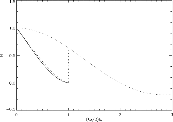
Because the optical OTF has an upper cut-off frequency k

(2.4-26), the same is

true for the total OTF. Figure 2.5-3 shows this for the case k

= k (k

= 0), 

= δ

=1/2k

, k

=D/(λb), which means that the Nyquist frequency k

nyq

=1/2

is equal

to the cut-off frequency and that the sampling condition (2.5-13) is just fulﬁlled.

According to (2.5-10), the OTF H

pix

,0) has the value 2/π ≈0.64 at the Nyquist

frequency. One can enhance this value if one decreases the pixel size δ

compared

to the pixel pitch 

. Then the total OTF corresponds better to that of the optical

system.

In Fig. 2.5-3 the OTF of the optics is plotted dashed, H

pix

,0) is the dotted

curve, and the total OTF H = H

opt

· H

pix

is the solid curve.

Fig. 2.5-3 Total OTF and OTFs of partial systems (description in the text)

2.5 Sampling 75

If the sampling distances are chosen as

Max

{

x,y

}

, (2.5-13)

the sampling condition is fulﬁlled and one can reconstruct the s patial signal f

pix

(x,y)

with the sampling values f

k,l

= f

pix

(kx,ly):

pix

(

x,y

)



pix

(

kx,ly

)

sin



x

(

x −kx

)



x

(

x −kx

)

sin



y

(

y − ly

)



y

(

y − ly

)

(2.5-14)

When the sampling condition is fulﬁlled, the values f

k,l

represent the whole signal

pix

(x,y) (they do so only approximately, of course, because there is only a ﬁnite

number of sampling values available). If it is not fulﬁlled, f

pix

(x,y) contains too high

frequencies and the sampling leads to the aforementioned aliasing errors, which may

change periodic signal parts in their spatial frequency and direction. For example,

the left-hand image in Fig. 2.5-4 shows a sinusoidal brightness distribution, which

was sampled at the brightly marked points, whereas the right-hand image displays

the brightness at the sampling points. One sees that the spatial frequency is too low

and the wave direction is wrong too.

The undersampling of periodic structures generates patterns which are a special

case of the well-known Moiré-patterns. These may arise when periodic structures

are observed through other periodic structures (e.g. a fence through ﬁnely woven

curtain).

Whereas insufﬁciently dense sampling points may lead to errors, unnecessarily

dense sampling points are not corruptive (of course, the amount of data is higher).

If the sampling distance has the maximum possible value 1/2k

then all sampling

points are necessary for the reconstruction of the whole function f

pix

(x,y). If only

one sampling value is absent, an exact reconstruction is no longer possible. But, if

Fig. 2.5-4 Aliasing

76 2 Foundations and Deﬁnitions

the sampling distance is smaller than 1/2k

, a certain redundancy is available, which

may be used to interpolate missing values, though this is not discussed here.

A detector array (Fig. 2.5-2) is not always used for imaging. If the imaging sys-

tem is moving relative to the scene, a detector line is sufﬁcient. Such a line sensor

with N pixels in the x-direction samples the intensity ﬁeld in the x-direction in the

same way as an array sensor. Sampling in the y-direction becomes possible because

of the relative motion of the sensor in that direction. Let f(x,y) be the intensity dis-

tribution in the image plane. When the sensor is moving with constant velocity v

(related to the image plane) in the y-direction, the intensity at a point (x

) (e.g.

the central point of a pixel) changes according to f(x

,y(t)) with y(t) = y

+ v·t.Ifthe

pixel is exposed during the time t (exposure time, integration time), the intensity

is integrated. As a result the signal

(

)

= t ·

t



f (x

+ν · t)dt

is generated in the detector element under consideration. This connection can also

be written as a linear system

(

)

= t ·

+v·t



mot

(

−y

)

·f

(

)

dy. (2.5-15)

with the PSF of motion or scanning

mot

(

)



v·t

for −vt ≤ ξ ≤ 0

0 elsewhere

(2.5-16)

Compared to f(x

), the intensity g(x

) is blurred in the y-direction (along-

track). The blur increases with the integration time t. It causes an asymmetry,

which can be minimized if integration time and pixel dimensions (δ

< δ

) are cho-

sen such that after the integration the effective pixel size in the y-direction δ

+v·t

is (approximately) equal to δ

Of course, a special sensor design is necessary for

this to be accomplished.

If the integration time is chosen such that the pixel shift during this time is equal

to the pixel size, it is called the dwell time t

dwell

. A point (x,y) of the optical signal

then crosses the pixel once during that time (it dwells inside the pixel). In most cases

one tries not to exceed the dwell time. Unfortunately, it is not possible to choose t

<< t

dwell

in most cases, because then the signal-to noise ratio becomes too low

(see Section 2.6).

If one uses two CCD lines (instead of one) with the second line shifted by

pixel with respect to the ﬁrst one (staggered array, Fig. 2.5-5), the ground sample

distance (GSD) can be halved in both directions (along track and across track).

But to enhance the geometric resolution too, it must be kept in mind that the PSF

2.5 Sampling 77

Fig. 2.5-5 Staggered array

of the optical system must be improved also (adequate enhancement of the cut-off

frequency k

With sensor arrays the same effect is achievable if the array is shifted in the x-

and y-directions by micro-scanning techniques. But this method is applicable only

if there is no motion between object and sensor during consecutive measurements.

Sometimes the geometric resolution of an optical system is equated with the

Ground Sampling Distance (GSD) (which corresponds to 

or 

in the image

plane). But in general this is not true! In Section 2.4, Rayleigh’s deﬁnition was used,

but this is not the ultimate limit of achievable resolution. If the signal-to-noise ratio

(SNR) is good, a central recess in the image of two neighbouring points which is

much smaller than the recess of 26% at the Rayleigh distance r

(see Fig. 2.4-8 and

(2.4-24)) can be detected. In the special case  = 

= 

= 1/2k

(no aliasing)

there is  =r

/2.42. Therefore, for good SNR, the GSD corresponds to a better res-

olution than r

and can serve as a rule of thumb value for the geometric resolution.

But ultimately the achievable resolution depends on the SNR.

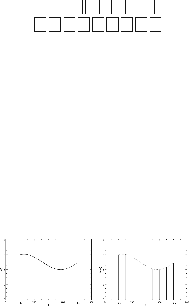
In short, the sampling of functions may be described as follows (Fig. 2.5-6). In

the two-dimensional case, sampling is the transition from f(x,y)tof

m,n

= f(m·x,

n·y). These functional characteristics are values from the continuum of real num-

bers. To process these numbers in digital computers they must be transformed to

digital numbers. This is done with the aid of analogue-to-digital converters or units

(ADC, ADU), which convert real numbers to integers. For instance, an 8-bit-ADU

converts an input signal (voltage) U

to a digital output value U

=n·U

(n =

0, 1, ...,2

–1), which corresponds to the digital number n. This operation may be

Fig. 2.5-6 One-dimensional sampling: continuous function f(t)(t

≤ t ≤ t

) → (time-) discrete

function f

= f(n·t) (n = n

,...,n

)

78 2 Foundations and Deﬁnitions

deﬁned in the following manner. If the input signal U

fulﬁlls the condition (n –

)· ≤ U

<(n +

)·, the output signal U

=n·U

, or the integer n is assigned

to U

. Of course, this operation causes a (digitisation) error (except if, by chance,

= n· holds), which is studied in the next chapter.

2.6 Radiometric Resolution and Noise

In the above sections the necessity of a good dignal-to-noise ratio (SNR) has

been mentioned. With good radiometric resolution the geometric resolution can

be enhanced. Thus radiometry and geometry are not independent characteristics.

To understand radiometric resolution correctly, the nature of random variables

and random processes must be understood. If there were no noise, the radiomet-

ric resolution, i.e. the possibility to discriminate neighbouring values of intensity,

would be arbitrarily large and one could separate any point sources that are close

together.

A random process ξ(t) is characterised by the fact that it is impossible to predict

future values of ξ(t) exactly. It is possible only to assign probabilities to such values.

The reason for the randomness of noise is the fact that the physical signal carriers

(photons, electrons etc.) perform random motions and are distributed randomly in

space. For example, the photons in a light beam are emitted by randomly distributed

emitting atoms or molecules in random moments of time. Therefore, the number

received by a detector element during a time interval t ﬂuctuates randomly. The

electrons responsible for the signal transfer inside a wire have a chaotic velocity

distribution (depending on the temperature of the wire) caused by interactions with

ions and other electrons. Thus signal ﬂuctuations are generated which are perceived

as noise during radio reception. Therefore the name “noise” was chosen for these

random processes.

Random ﬁelds ξ(x,y,...) are two- or multi-dimensional generalisations of ran-

dom processes, whereas random variables are represented by numbers ξ

, ξ

... , ξ

. Here, the theory of random processes can be presented only very

brieﬂy.

Because optoelectronic imaging sensors are sampling systems, the following

remarks are focused on a short discussion of random variables (e.g. ξ

k,l

= ξ(x

)

as sampling values of the random ﬁeld ξ(x,y)).

Let ξ be a random variable which can take real numbers x. These values are

described by the probability density p

(x). p

(x)dx is the probability of the event that

the value of ξ is a real number in the interval [x,x+dx] as the result of an experiment.

Then the probability of the event that ξ takes a value x inside the interval x

≤ x ≤

is given by

{

≤ x ≤ x

}



(

)

dx. (2.6-1)

2.6 Radiometric Resolution and Noise 79

Because it is certain that ξ takes a value inside –∞ < x <+∞ and because

the unit probability is assigned to an event that will take place with certainty, the

relationship

+∞



−∞

(

)

dx = 1. (2.6-2)

holds.

The function p

(x) allows one to deﬁne the so-called expected values. Let f(ξ)

be any function of the random variable ξ. Then the expected value of f(ξ)is

given by





+∞



−∞

(

)

(

)

dx. (2.6-3)

If one carries out N experiments with the result that the random variable f(ξ) takes

the values f

,...f

then one can calculate the arithmetic mean value

f =



n=1

. (2.6-4)

If N is large then

f is near to f with high probability. Therefore, the expected

value is also called the statistical mean value.

In the following the expected value





+∞



−∞

x · p

(

)

dx (2.6-5)

of the random variable ξ itself and the expected value of squared variable (ξ –

ξ)

(

ξ −





)

+∞



−∞

(

x −





)

·p

(

)

dx, (2.6-6)

which is the variance of the random variable ξ, are used. The standard devi-

ation σ

(the square root of the variance) is a measure of the deviation of ξ

from the mean value ξ and therefore a measure of the width of the probability

density p

(x).

The mean energy of the black body radiation of temperature T inside the wave-

length interval [λ, λ+λ] is considered by way of an example. This is received

during the integration time t by a detector element. It is proportional to Planck’s

function B

(T) (see Section 2.2). B

(T) is not a random variable: it characterises the

mean radiance of the black body radiation! Therefore, all radiometric quantities con-

sidered up to now must be understood as statistical mean values. The values obtained

as the results of measurements ﬂuctuate around these mean values. The standard

80 2 Foundations and Deﬁnitions

deviation σ is a measure of that ﬂuctuation. Therefore, it is useful to characterise

the quality of a signal by the signal-to-noise ratio

SNR =





. (2.6-7)

Let E = ·t be the energy which a detector element receives during the inte-

gration time t ( is the power of that radiation; see Section 2.2). If the detector

is linear (a condition well fulﬁlled by CCD sensors) then the sensor output signal

U is proportional to E: U = K · E. During a measurement the (noisy) value U =

U + δU is observed. Here, δU is a random variable with the mean value δU=

0 and standard deviation σ

. It is assumed that the noise δU is generated in the

detector and/or the read-out electronics and that the input signal (the radiation) is

noise-free (which means that the photon noise, which is developed in (2.6-20), (2.6-

21), (2.6-22), (2.6-23) and (2.6-24), can be neglected). Then, an error δE = δU/K

and an error δ = δU/(K·t) may be attributable to the random error δU. Those

random variables have the standard deviations σ

= σ

/K and σ



= σ

/(K·t),

respectively. They are measures of the quality with which the radiometric variable

under consideration can be measured and deﬁne the achievable radiometric resolu-

tion. In particular, σ



is called the Noise Equivalent Power (NEP). In this way, the

radiometric resolution of other radiometric variables such as the radiance may also

be estimated. For instance, if one measures the r adiation in the wavelength interval

λ then according to (2.2-9) the relationship

 = K

·L

; K

·cos

(

)

·τ

·λ

is true, and it holds that σ

Lλ

= σ

/(K

·K·t).

If the connection between U and E is non-linear (for CMOS sensors, for exam-

ple), the radiometric resolution of E (and also of  or L

) may be determined if the

probability density p

(u) of the random variable U is known. Let the connection

between E and U be given by E = f(U). Then, according to (2.6-3) and (2.5-6) the

following relationships hold:

(

E −





)





(

)

−







·p

(

)

du, (2.6-8)

and







(

)

·p

(

)

du. (2.6-9)

The linear relationship E = U/K is a special case of E = f(U). For practical

purposes (with weak noise) the simpler relationships

≈





(





)



·σ

(2.6-10)