Stacey F.D., Davis P.M. Physics of the Earth
Подождите немного. Документ загружается.

//FS2/CUP/3-PAGINATION/SDE/2-PROOFS/3B2/9780521873628C09.3D
–
117
– [117–134] 13.3.2008 10:36AM
9
The satellite geoid, isostasy, post-glacial
rebound and mantle viscosity
9.1 Preamble
Gravity observations are referred to an equipo-
tential surface, termed the geoid, for which sea
level is a close approximation. We can picture the
geoidal surface in continental areas as following
the water level in hypothetical narrow canals
connected to the oceans. For a non-rotating
planet in hydrostatic equilibrium the geoid
would be a sphere but rotation deforms it to an
oblate ellipsoid. For several reasons discussed in
Section 6.4 the Earth is slightly more elliptical
than equilibrium theory would suggest. One
reason is the depression of polar regions by for-
mer glaciation, from which recovery is incom-
plete and the continuing rebound gives a clue to
the viscosity of the mantle. There are heteroge-
neities at all levels, the most obvious of which
are seen at the surface as continents and oceans,
but the effect of the continent–ocean structure
on the geoid is barely discernible and very much
less than if the continents were superimposed
on an otherwise uniform Earth. On a continen-
tal scale the surface features are very nearly in
hydrostatic balance . This is the principle of
isostasy.
Features of the gravity field on a scale
larger than 1000 km are discerned more effec-
tively by studying perturbations of satellite
orbits than would be possible from surface
observations. With progressive improvements,
satellite techniques have been used to distinguish
increasingly fine features, although for explora-
tion of local anomalies surface observations
on land must still be used, sometimes in combi-
nation with satellite data. The shape of the sea
surface is observed by satellite altimetry, radar
reflections to satellites. It follows the geoid quite
closely and shows finer scale details than could
be inferred from orbital motion.
Gravitational perturbations of satellite orbits
are analysed in terms of spherical harmonics
(Appendix C). In Section 6.2 we consider just
the centred mass and ellipticity. The effect of
ellipticity is smaller than the central gravita-
tional attraction by a factor of 1000 for satellites
in low orbits, r a. The higher terms in a more
general harmonic expansion, representing finer
details of the field that we now consider, are
smaller still, by another factor 1000. For this
purpose the harmonic terms are fully norma-
lized, as defined by Eqs. (C.13) and (C.14) in
Appendix C, so that the mean square values
over the surface of a sphere are unity. This
means that the coefficients
C
m
l
and
S
m
l
, represent-
ing departures from sphericity, relate directly to
the amplitudes of the features represented.
Referred to fully normalized harmonics the
ellipticity coefficient is not J
2
(Eq. (6.14)), but
C
0
2
¼J
2
=
ffiffiffi
5
p
. However, if interest is restricted
to ellipticity, then J
2
is used.
For more than two decades, satellite measure-
ments of J
2
have been precise enough to observe
a slow decrease with time,
_
J
2
¼2.8 10
11
per
year. The rate is clearly greater than can be

//FS2/CUP/3-PAGINATION/SDE/2-PROOFS/3B2/9780521873628C09.3D
–
118
– [117–134] 13.3.2008 10:36AM
explained by tidal braking of the Earth’s rotation
(Section 8.4) and is attributed to post-glacial
rebound, although the adequacy of this to
explain the total
_
J
2
remains to be confirmed.
The transfer of mass into the depressed areas
from lower latitudes causes a decrease in the
axial moment of inertia, C, and this is apparent
from the corresponding decrease in J
2
. Unlike
tidal friction, which transfers rotational angu-
lar momentum to the lunar and solar orbits,
rebound conserves rotational angular momen-
tum and so causes spin-up, partially offset-
ting the rotational slowing by tidal friction
(Section 6.4).
As mentioned in Section 6.4,
_
J
2
cannot be
used directly to infer relaxation of excess J
2
,
because the excess attributable to glaciation
cannot be separated from other, unrel ated
components. Instead
_
J
2
is interpreted as a
response to a known history of ice loading.
Of the areas of former deep glaciation, where
rebound continues at an observable rate, the
two that have been studied in closest detail are
Fennoscandia, centred on the Gulf of Bothnia,
and Laurentia, centred on Canada . We con-
centrate attention on Laurentia, which is
much bigger and, according to Peltier’s (2004)
ice model, accounts for as much as 2/3 of the
global de glaciation. Antarctica ranks second,
although it still holds more ice than it is es-
timated to have lost. We use L aurentia to
estimate the fraction of
_
J
2
that is explained by
it, with the conclusion is that there is a bi gger
ellipticity effect than is explained by the docu-
mented areas of rebound.
From a fundamental perspective the most
interesting conclusion of rebound studies
is the viscosity of the mantle and its depth
dependence. These studies assume that the
mantle rhe ology is linea r, a s for a Newtonian
viscous fluid. This assumption is insecure, and
the possibility of non-linear rheology is con-
sidered in Section 10.6. Non-linearity means
that different values of effective vi scosity
would apply to processes with different strain
rates. In applying the rebound estimate of vis-
cosity to mantle conv ection in Section 1 3.2,
we conclude that these two phenomena are
consistent with similar values of viscosity.
However, the strain rates for plate motion
and post-glacial rebound are a lso similar. The
same value of effective viscosity would be
expected for both, whether or not the mantle
theology is linear. This gives confidence that
both convection and rebound are satisfactorily
explained, but the question of linearity remains
unanswered.
9.2 The satellite geoid
To a first approximation the effect of the Earth’s
gravity on a satellite is given by the first term
of Eq. (6.2) or (6.13), which describes the force
maintaining the satellite on an elliptical orbit
(Appendix B). The following discussion considers
first the effect of the second term in these equa-
tions and then higher order terms. As considered
in Section 7.2, the second term causes a mutual
precessional torque between the Earth and the
satellite. For a man-made satellite the effect on
the Earth is negligible, but the satellite orbit
precesses at a rate that provides a measure of
the ellipticity coefficient J
2
(Eq. (6.14)). This is
referred to as a regression of the nodes of the
orbit, that is a progressive drift of the points at
which it crosses the orbital plane (as seen by an
observer fixed in space, not rotating with the
Earth). Equations describing this process follow
closely those used in Section 7.2 for precession
of the Earth.
Considering a satellite in an orbit of radius
r, inclined at an angle i to the equatorial plane,
we may rewrite Eq. (7.10) to give the mean
torque over a complete orbit, acting on the
satellite,
L ¼
3
2
Gm
r
3
Ma
2
J
2
cos i sin i; (9:1)
where m is the satellite mass and M is the Earth’s
mass. This torque acts on the component of the
orbital angular momentum that is perpendicular
to the Earth’s axis,
p
?
¼ mr
2
!
S
sin i; (9:2)
118 THE GEOID, ISOSTASY AND REBOUND

//FS2/CUP/3-PAGINATION/SDE/2-PROOFS/3B2/9780521873628C09.3D
–
119
– [117–134] 13.3.2008 10:36AM
where !
S
is the orbital angular speed of the satel-
lite. The mean angular rate of the orbital preces-
sion, observed as a steady regression of the nodes
of the orbit, that is the positions in space where
they cross the equatorial plane, is the ratio of the
torque to the angular momentum component on
which it acts,
!
P
¼
L
p
?
¼
3
2
GMa
2
J
2
r
5
!
S
cos i: (9:3)
This simplifies by applying Kepler’s third law
!
2
S
r
3
¼ GM
to the orbit:
!
P
¼
3
2
!
S
a
2
r
2
J
2
cos i: (9:4)
Thus the angular change per orbital revolution
in the position of a node is DO, given by
O
2p
¼
!
P
!
S
¼
3
2
a
2
r
2
J
2
cos i: (9:5)
For a close orbit (at r ¼1.03 a) inclined at i ¼458,
O ¼0.388.
Equation (9.5), or a more g eneral version for
an elliptical orbit, suffices for a determination
of J
2
to an accuracy of order 1 part in 1000, but
for greater accuracy higher harmonics in the
gravitational potentia l must be taken into
account. Variations with longitude (tesseral har-
monics, as given by Eq. (C.15) in Appendix C,
with m 6¼0) are averaged out by taking a long
record of nodal r egression, but all zonal har-
monics (with m ¼0 and no longitude d epend-
ence) contribute to the long-term average of
DO. The contributions depend in different
ways on the inclinations and radii of th e
orbits, so that data from several satellites are
required to separate them. Detailed observa-
tions of elliptical orbits also provide additional
information.
In applying Eq. (C.15) to the general problem
of the geoid, only the unprimed coefficients,
representing sources of internal origin, are of
interest.Itisconvenientalsotowritethel ¼0
term, representing the central mass, separately,
and t o note that l ¼1 gives an asymmetrical
potential and that it vanishes by the selection
of the centre of mass of the Earth as the coor-
dinate origin. Then, by normalizing the sum of
all terms to (GM/r), the potential in standard
form, with fully normalized coefficients
(Eq. (C.13)), is
V ¼
GM
r
1 þ
X
1
l¼2
a
r
l
X
l
m¼0
p
m
l
sin ðÞ
(
C
m
l
cos ml þ S
m
l
sin ml
hi
)
: ð9:6Þ
Care is required with signs, as well as normal-
ization, in the application of this equation.
Thus, for example,
C
0
2
¼J
2
=
p
5, as mentioned
in Section 9.1.
Tesseral harmonics (with m 6¼0) in the
gravitational potential cause shorter-period
variations in satellite orbits (such as an oscilla-
tion in the rate of nodal regression) than do
the zonal harmonics. More detailed observa-
tions are required to measure them. It follows
also that they are less accurately d etermined.
Nevertheless, there have been numerous inde-
pendent studies and they have converged to
good agreement for harmonics to l 50. Values
of geo id coe fficients to degree and order (8,8)
are listed in Table 9.1, and Fig. 9.1 is a map of
geoidal elevation obta ined from coefficients
to degree and order (50,50). Rapp and Pavli s
(1990) reported a calculation of geoid coeffi-
cients to harmonic degree 360 with a full
geoid map.
The spherical harmonic representation of the
geoid is particularly appropriate for analysis of
its broad features and follows naturally from the
study of perturbations in satellite orbits, which
provide the most accurate measure of the low-
degree terms. Spherical harmonic expansions
become cumbersome when extended to high
harmonic degrees, l, because, for l 2, the num-
ber of coefficients varies as (l
2
þ2l 5). There
is also a problem of uneven coverage of the
Earth when satellite orbit data are supplemented
by surface measurements to fill in the fine
details. However, satellite altimetry, the tim-
ing of radar reflections to satellites from the
sea surface, has given considerable detail i n
9.2 THE SATELLITE GEOID 119
//FS2/CUP/3-PAGINATION/SDE/2-PROOFS/3B2/9780521873628C09.3D
–
120
– [117–134] 13.3.2008 10:36AM
0° 30° 60° 90° 120° 150° 180° 210° 240° 270° 300° 330° 360°
0° 30° 60° 90° 120° 150° 180° 210° 240° 270° 300° 330° 360°
–60° –60°
–30° –30°
0° 0°
30° 30°
60° 60°
–80
–80
–60
–6
0
–60
–20
–20
–20
–40
–20
–20
–40
–20
–40
–20
–20
0
–40
0
0
0
0
0
0
20
–40
–40
–40
–20
0
20
20
20
20
20
20
20
20
0
0
20
40
40
60
40
40
60
60
20
0
–20
–60
–40
–20
0
0
20
40
40
20
0
–40
–20
20
40
40
60
60
0
–40
–40
–20
0
20
20
20
–40
0
0
0
–40
–20
–20
20
60
–40
0
–20
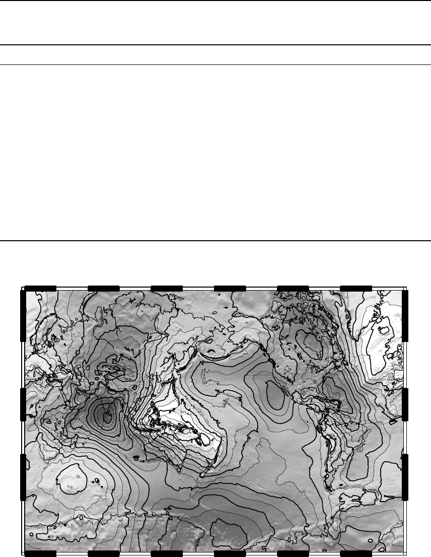
FIGURE 9.1 Contours of geoid height (in metres), relative to the reference ellipsoid (f ¼1/298.257). Courtesy of
David Sandwell.
Table 9.1 Spherical harmonic coefficients of the Earth’s gravitational potential to degree and
order (8,8), from a more extensive set by Lerch et al. (1994). For each (l,m) the coefficients are
C
m
l
followed by
S
m
l
, in units of 10
6
, as in Eq. (9.6) and defined in Appendix C
l\m 01 2 3 4 5 6 7 8
2 – – 2.439 – – – – – –
484.165 1.400
3 0.957 2.029 0.904 0.720 – – – – –
0.249 0.619 1.414
4 0.539 0.536 0.349 0.991 0.188 – – – –
0.473 0.664 0.201 0.309
5 0.069 0.061 0.655 0.452 0.296 0.175 – – –
0.096 0.325 0.217 0.050 0.668
6 0.148 0.076 0.052 0.057 0.088 0.267 0.010 – –
0.026 0.376 0.009 0.472 0.536 0.237
7 0.090 0.280 0.323 0.251 0.275 0.002 0.359 0.001 –
0.096 0.096 0.212 0.128 0.019 0.152 0.024
8 0.047 0.023 0.073 0.018 0.244 0.025 0.065 0.069 0.123
0.060 0.069 0.087 0.068 0.088 0.309 0.076 0.122
120 THE GEOID, ISOSTASY AND REBOUND
//FS2/CUP/3-PAGINATION/SDE/2-PROOFS/3B2/9780521873628C09.3D
–
121
– [117–134] 13.3.2008 10:36AM
oceanic areas. It demonstrates the close corre-
spondence of the fine structure of the geoid to
tectonic features of the Earth (Fig. 9.2), as
reflected in the sea floor to pography, which
the sea-surface geoid mimics.
The relationship of the low-degree harmonic
terms to the internal structure and dynamics
of the Earth is less obvious. The spectrum o f
harmonic degree amplitudes plotted in Fig. 9.3
indicates that the low degrees represent
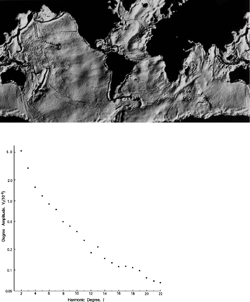
FIGURE 9.2 The mean sea level, as mapped by satellite altimetry, reflects the geoid in oceanic areas.
Reproduced from Cazenave (1995).
FIGURE 9.3 Degree amplitudes, as
defined by Eq. (9.7), of the spherical
harmonic coefficients of the geoid
listed by Lerch et al. (1994). Values
corresponding to the equilibrium
ellipticity have been subtracted
from
C
0
2
and
C
0
4
.
9.2 THE SATELLITE GEOID 121

//FS2/CUP/3-PAGINATION/SDE/2-PROOFS/3B2/9780521873628C09.3D
–
122
– [117–134] 13.3.2008 10:36AM
deeper features than those responsible for the
detailsseeninFig.9.2.Sincesphericalhar-
monics are orthogonal functions, the total
amplitude of all harmonic terms of degree l,
taken together, is
V
l
¼
X
l
m¼0
C
m
l
2
þ S
m
l
2
()
1=2
; (9:7)
and this is the function plotted in Fig. 9.3. V
l
is
the rms amplitude (square root of spectral
power) of geoid undulations with wavelength
(2pR
E
/l), where R
E
is the Earth’s radius. The spec-
trum in Fig. 9.3 is very ‘red’, that is amplitude
increases with wavelength, or l
1
. This is indica-
tive of deep mantle sources. The approximately
linear decrease in log V
l
with l over the range l ¼4
to 16 is suggestive of a spectrally ‘white’ source
at a radius at which d(lnV
l
)/dl would be zero. This
would put it well into the lower mantle.
Although a source at a single depth could not
be physically realistic, and density heterogene-
ities are widely distributed, the broad-scale
features of the satellite geoid indicate that the
heterogeneities extend deep into the lower
mantle.
If such an analysis is extended to higher
harmonic degrees, then it is obvious that the
spectral ‘redness’ cannot persist indefinitely.
Deep-seated contributions to high-degree com-
ponents of the geoid cannot be seen at the
surface and effects of shallower sources becom e
dominant.
9.3 The principle of isostasy
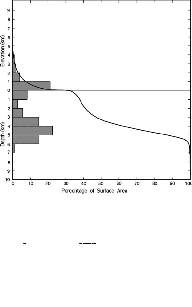
The distribution of elevations of the Earth’s solid
surface is strongly bimodal, as illustrated in
Fig. 9.4. Most of the surface is either of continen-
tal type, with an elevation within 1 km of sea
level, or of oceanic type, 4 to 5 km below sea
level. Taking the average density difference
between the continental crust and sea water to
be 1750 kg m
3
, the continents have a mass
excess, relative to the oceans, of 8 10
6
kg m
2
above the level o f the ocean floor. Such a
mass excess is not evident in the broad scal e
features of the geoid in Fig. 9.1. Thus thi s
mass is compensated by continent al ‘roots’
of material with lower density than that of
the sub-oceanic mantle. This is the principle
of isostasy, first stated in the mid-nineteenth
century whe n it was recognized th at the gra-
vitational deflection of the vertical by the
Himalaya mo untains was much less than if
theyweresimplyaprotrusiononanother-
wise spherically layered Earth. As we now
know from seismic studies, the continental
crust is typical ly 35 km to 40 km thick (60
to 75 km u n d e r t h e Himalaya), whereas the
oceanic crust is only 7 km thick, and both over-
lie the denser mantle. We consider a plausible
reason for the continental thickness at the end
of this section, and, in Section 23.2 make use
of the idea that it has been constant as the
crust developed by differentiation from the
mantle.
For an idea of the effect of continents on t he
geoid, consider an idealized pair of circular con-
tinents on a spherical Eart h, as in Fig. 9.5. Thi s
simple geometry allows their broad scale (ellip-
soidal) deformation of the geo id to be calculated
from their moments of inertia by Eq. (6.13).
In case (a) the moments of inertia of the Earth
about axes 1 and 2 differ only by the moments
of inertia I
1
and I
2
of the continents a bout these
axes. In the approximation that the radii, r,of
the continents, as well as their thicknesses, h,
are much less than t he radius of the Earth,
h r a,
I
1
2 pr
2
h
c
r
2
=2; (9:8)
I
2
2
ð
aþh
a
pr
2
c
x
2
dx 2pr
2
c
a
2
h; (9:9)
so that
I
1
I
2
2pr
2
c
a
2
h: (9:10)
Thus
J
2
¼
I
1
I
2
Ma
2
2p
c
r
2
h=M; (9:11)
122 THE GEOID, ISOSTASY AND REBOUND
//FS2/CUP/3-PAGINATION/SDE/2-PROOFS/3B2/9780521873628C09.3D
–
123
– [117–134] 13.3.2008 10:36AM
and by Eq. (6.20), with rotation not considered,
f ¼
3
2
J
2
3p
c
r
2
h=M
9
4
r
2
h
a
3
c
; (9:12)
where
is the mean density of the Earth. The
negative flattening means a prolate elongation
along axis 1. The geoid elevation, h
g
, on this axis,
relative to axis 2, is a fraction of the continental
elevation, h, given by
h
g
h
¼
fa
h
¼
9
4
r
2
a
2
c
: (9:13)
Taking r ¼2500 km as representative of a conti-
nent, and
c
¼1750 kg m
3
as the density differ-
ence between the continent and sea water,
h
g
0:11h: (9:14)
If this analysis were applicable to the real
Earth, we would see systematic differences in
geoid heights between centres of continents and
oceans of order 0.11 4500 m ¼500 m. Not only
are geoid height variations very much smaller
than this, but the variations that are observed
(Fig. 9.1) are not obviously related to the continent–
ocean structure. On a continental scale isostatic
balance is closely maintained, although rigidity
of the lithosphere supports isostatic anomalies
on a scale of order 100 km.
Now consider the continental model in
Fig. 9.5(b) and require that it cause no geoid
ellipticity. This requirement is satisfied by mak-
ing the moments of inertia of the continents
equal to that of the oceanic crust and mantle
that would replace them to produce a spherically
symmetrical Earth:
FIGURE 9.4 The hypsographic curve – the characteristic distribution of the elevations of the solid surface – with a
histogram of areas in 1000 m elevation intervals.
9.3 THE PRINCIPLE OF ISOSTASY 123
//FS2/CUP/3-PAGINATION/SDE/2-PROOFS/3B2/9780521873628C09.3D
–
124
– [117–134] 13.3.2008 10:36AM
2
ð
aþh
ad
pr
2
c
x
2
dx ¼2
ð
at
ad
pr
2
m
x
2
dx
þ 2
ð
a
at
pr
2
o
x
2
dx:
(9:15)
With the conditions d, t, h a, this gives
c
h þ dðÞ¼
m
d tðÞþ
o
t: (9:16)
which is a statement of the principle of isostasy,
that the total masses in all vertical columns (of
unit area) are the same.
Equation (9.16) incorporates both of the r ival
hypotheses that were inspired by the evidence
that the Himalaya are isostatically balanced.
They express alternative methods by which iso-
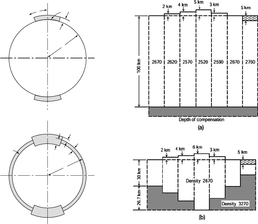
stasy may be achieved, as in Fig. 9.6. In 1854
J. H . Pratt suggested that the higher parts of
the crust were elevated by virtue of their
lower densities, with a common compensation
depth, as in Fig. 9.6(a), and the following year
G. B. Airy proposed the structure represented by
Fig. 9.6(b). He visualized the crustal masses as
logs, all of the same density, floating in water.
Axis 1
Axis 1
r
h
ρ
c
ρ
c
ρ
o
ρ
m
a
Axis 2
Axis 2
a
d
h
t
(a)
(b)
FIGURE 9.5 Simple models of a symmetrical pair
of continents, illustrating their effect on the geoid.
(a) Continents superimposed on an otherwise spherically
symmetric Earth. (b) Continents of density
c
overlying
a mantle of density
m
and isostatically balanced with an
oceanic crust of density
o
.
FIGURE 9.6 Isostatic compensation according to
(a) J. H. Pratt and (b) G. B. Airy, with numerical values of
density by W. A. Heiskanen. Continents, ocean basins and
mountain ranges are balanced by either of these principles.
Crustal structure corresponds more nearly to (b).
124 THE GEOID, ISOSTASY AND REBOUND
//FS2/CUP/3-PAGINATION/SDE/2-PROOFS/3B2/9780521873628C09.3D
–
125
– [117–134] 13.3.2008 10:36AM
A log appearing higher out of the water than
its neighbours must extend correspondingly
deeper. Isostatic balance of the continents
would be achieved by Pratt’s principle if d ¼t in
Eq. (9.16), so that
c
h þ t
ðÞ
¼
o
t; (9:17)
or by Airy’s principle if
c
¼
o
, in which case
c
h þ d tðÞ¼
m
d tðÞ: (9:18)
Both principles contribute to the isostatic bal-
ance of continents and mountain ranges, the
Airy principle being generally the more
important.
Now we return to a consideration of Fig. 9.4.
The continental crust is dominated by acid
(Si rich) rocks that are less dense than the
ocean floors, with which they are isostatically
balanced. The continents do not spread out to
cover the whole Earth uniformly, but are effec-
tively swept clear of 60% of the surface area by
the continuous renewal of the ocean floors. The
continental material washed into the oceans as
sediment is returned by underplating and via
subduction zones and volcanism. What deter-
mines the thickness of the continental crust
and thus the area that it occupies? As illustrated
by Fig. 9.4, most of the continental area is close
to sea level and this is a clue that it is reduced to
that level by erosion, which has little effect on
lowlands and continental margins. Higher ele-
vations are maintained by tectonic activity, but
erode rapidly, and so are relatively young. It
is not fortuitous that most of the continental
area is close to sea level, but a consequence of
the erosion–regeneration cycle. Thus it is sea
level itself that controls the continental thick-
ness. This argument is used in Section 23.2 to
support the assumption that, in the remote past,
when less continental material had accumu-
lated, its thickness was little different from the
present time, but its area was smaller. The
assumption is necessarily only an approxima-
tion, because, even assuming a constant volume
of sea water, smaller continents would mean
lower sea level.
9.4 Gravity anomalies and the
inference of internal structure
Gravity anomalies are departures of observed
gravity from the reference latitude variation in
Eq. (6.38). They are of interest as indicators of
internal structure, but it is important to recog-
nise that there can be no unique solution to the
problem of calculating internal density varia-
tions from observations of gravity on or above
the surface. The forward problem of calculating
gravity from any specified mass distribution is
unambiguous, but there is, in principle, an infin-
ite number of density distributions that could
explain a gravity anomaly pattern. The range is
restricted by plausibility, by setting up density
models that mimic the observed gravity. This is
aided by processing gravity data to represent
anomalies in different ways. We refer to three
types of anomaly presentation: free-air, Bouguer
and geoid. The first two are mentioned in
Section 6.3 and geoid anomalies are illustrated
inFigs.9.1and9.2.Herewetakeacloserlook
at the implications and assumptions, noting
the essential point that gravity observations
on a surface of variable elevation would be dif-
ficult to interpret directly and there are alter-
native ways of transposing them to the geoidal
surface.
The free-air gradient means the radial variation
of gravity above ground level. The global ave-
rage value is 0.3086 mGal m
1
(3.086 10
6
s
2
).
A free-air anomaly is the departure from the
standard gravity formula (Eq. (6.38)) on the
geoid (or mean sea level), calculated by assum-
ing this gradient to apply from a sur face point of
observation. Usually, but not necessarily, the
small latitudinal and local variations in the gra-
dient are neglected. In principle it means calcu-
lating the gravity that w ould be observed o n the
geoid if all of the mass above it were collapsed
belowit.Ofcourse,thisisunsatisfactoryin
areas of more than very limited topography
and topographic corrections are generally
needed for the calculated anomalies to be use-
ful. Then the resulting free-air anomalies are
indications of concentrations or deficiencies in
9.4 GRAVITY AND INTERNAL STRUCTURE 125
//FS2/CUP/3-PAGINATION/SDE/2-PROOFS/3B2/9780521873628C09.3D
–
126
– [117–134] 13.3.2008 10:36AM
density below the points of observation. On
scales smaller than 100 km or so the strength
(or very high viscosity) of the lithosphere can
support departures from isostatic balance that
are apparent as free-air anomalies, notably at
the margins of continents. This is an indication
of what is known as the depth of compensation,
that is the depth below which viscosity is low
enough to equalize pressures (or below which
homogeneity can be assumed). As we see from
the global analysis in Section 9.3, on a larger
scale isostasy prevails and this means equality
of the masses in all vert ical columns, so that
free-air anomalies are weak. However, on a
scale of several thousand kilometres free-air
anomalies larger than those at intermediate
scales are apparent from the geoid plot in
Fig. 9.1. They are attributed to heterogeneity of
the lower mantle. This is possible because,
although the relatively low viscosity of the
asthenosphere explains the isostatic balance
at intermediate scales (200–2000 km) it does
not nullify the effect of irregular masses in
the more viscous lower mantle. These masses
must be deep as they are not evident at the
intermediate scale.
For the interpretation of local geol ogical
structures it is often more effective to calcu-
late gravity on the geoid assuming complete
removal of all material above it, instead of col-
lapse to the geoid. This gives Bouguer anoma-
lies. In the simplest cases, with no allowance
for topography or heterogeneity, the removed
material is assumed to be an extensive slab of
uniform thickness equal to the height at the
point of measurement. The gravity due to a
slab of thickness h,density and infinite hori-
zontal extent, is (see Problem 9.2)
g ¼ 2pGh; (9:19)
and is independent of distance from it. Thus,
calculation of gravity on the geoid by the
Bouguer method means downward extrapola-
tion from elevation h by a Bouguer gradient
which is equal to the free-air g radient minus
g/h ¼2pG. Commonly a standard density,
2670 kg m
3
, is used for this purpose and
then the Bouguer gradient is 0.1967 mGal m
1
(1.967 10
6
s
2
), about 2/3 of the free-air gra-
dient. If the density of the surface layers is
knownthenitisobviouslybettertousethat
rather than the standard value and, as with
free-air calculations, topographic corrections are
usually necessary. Bouguer anomalies are of inter-
est in studies of local crustal structure because
they reflect density variations immediately
below the geoid. On a continental scale Bouguer
anomaly maps show systematic lows over conti-
nents because, by Eq. (9.19), they differ from free-
air anomalies by 2pGh at height h and on this
scale isostatic balance prevails, making free-air
anomalies small.
The purpose of free-air and Bouguer anom-
aly maps is to remove the effect of ground ele-
vation, which obscures the underlying density
variations. They are complementary, giving dif-
ferent information, and it is instructive to have
both.Thethirdmethodistousegeoidanoma-
lies, that is variations in the height of the geoid,
taking advantage of satellite observations of
large-scale features, as in Fig. 9.1, and giving a
different perspective on isostasy. The general
idea can be understood from a simple example.
If, in a broad, topographically featureless area
of average d ensity r,wehaveapatchwithden-
sity ( þD) underlying a layer of equal thick-
ness but density ( D) then, by the argument
in Section 9.3 the patch would be isostatically
balanced. However, it would nevertheless
appear as a geoid anomaly. The reason is that
the deeper, denser layer gives enhanced gravity
within and above it and, since this is the gra-
dient of gravitational potential, in integrating
upwards from the depth of compensation
(below the patch) t he potential corresponding
to the geoid is reached at a lower level than in
areas outside the patch. A density dipole of this
form gives a geoid low. Conversely, if a denser
layer overlies a less dense one it gives a geoid
high. Thus a geoid anomaly gives information
about the depth distribution of mass and not
just its total. In this simple, plane layered
model the geo id anomaly, DN (metres), is
related to the depth dependence of the density
anomaly by integrating Eq. (9.19) through it
from the depth of co mpensation to the geoid
potential,
126 THE GEOID, ISOSTASY AND REBOUND