Stewart J. Calculus

Подождите немного. Документ загружается.

about the -axis. Therefore, from Formula 7, we get

! 2

""cos t#

]

! 4

! 2

sin t dt

! 2

r sin t ! r dt! 2

r sin t

"sin

t # cos

t# dt

S !

r sin t

""r sin t#

# "r cos t#

672

|| ||

CHAPTER 11 PARAMETRIC EQUATIONS AND POLAR COORDINATES

19. ,

20. ,

;

21. Use a graph to estimate the coordinates of the rightmost point

on the curve , . Then use calculus to ﬁnd the

exact coordinates.

;

22. Use a graph to estimate the coordinates of the lowest point

and the leftmost point on the curve , .

Then ﬁnd the exact coordinates.

;

23–24 Graph the curve in a viewing rectangle that displays all

the important aspects of the curve.

24. ,

Show that the curve , has two

tangents at and ﬁnd their equations. Sketch the curve.

;

26. Graph the curve , to

discover where it crosses itself. Then ﬁnd equations of both

tangents at that point.

27. (a) Find the slope of the tangent line to the trochoid

, in terms of . (See

Exercise 40 in Section 11.1.)

(b) Show that if , then the trochoid does not have a

vertical tangent.

28. (a) Find the slope of the tangent to the astroid ,

in terms of . (Astroids are explored in the

Laboratory Project on page 665.)

(b) At what points is the tangent horizontal or vertical?

29. At what points on the curve , does

the tangent line have slope ?

30. Find equations of the tangents to the curve ,

that pass through the point .

Use the parametric equations of an ellipse, ,

, , to ﬁnd the area that it encloses.0 +

+ 2

y ! b sin

x ! a cos

31.

"4, 3#y ! 2t

# 1

x ! 3t

# 1

y ! 1 # 4t " t

x ! 2t

y ! a sin

x ! a cos

y ! r " d cos

x ! r

" d sin

y ! sin t # 2 sin 2tx ! cos t # 2 cos 2t

"0, 0#

y ! sin t cos tx ! cos t

25.

y ! 2t

" tx ! t

# 4t

" 8t

y ! t

" tx ! t

" 2t

23.

y ! t # t

x ! t

" 2t

y ! e

x ! t " t

y ! 2 sin

x ! cos 3

y ! sin 2

x ! 2 cos

1–2 Find .

1. , 2. ,

3–6 Find an equation of the tangent to the curve at the point cor-

responding to the given value of the parameter.

3. , ;

4. , ;

, ;

6. , ;

7– 8 Find an equation of the tangent to the curve at the given

point by two methods: (a) without eliminating the parameter and

(b) by ﬁrst eliminating the parameter.

7. , ;

8. , ;

;

9–10 Find an equation of the tangent(s) to the curve at the given

point. Then graph the curve and the tangent(s).

9. , ;

10. , ;

11–16 Find and . For which values of is the

curve concave upward?

, 12. ,

13. , 14. ,

15. , ,

16. , ,

17–20 Find the points on the curve where the tangent is horizon-

tal or vertical. If you have a graphing device, graph the curve to

check your work.

17. ,

18. , y ! 2t

# 3t

# 1x ! 2t

# 3t

" 12t

y ! t

" 12tx ! 10 " t

y ! cos tx ! cos 2t

y ! 3 cos tx ! 2 sin t

y ! t " ln tx ! t # ln ty ! t # e

x ! t " e

y ! t

" 1x ! t

" 12ty ! t

# t

x ! 4 # t

11.

y!dx

dy!dx

""1, 1#y ! sin t # sin 2tx ! cos t # cos 2t

"0, 0#y ! t

# tx ! 6 sin t

(

)

y ! sec

x ! tan

"1, 3#y ! t

# 2x ! 1 # ln t

! 0y ! sin

# cos 2

x ! cos

# sin 2

t ! 1y ! t " ln t

x ! e

t ! 1y ! 1 # t

x ! t " t

t ! "1y ! t

# tx ! t

# 1

y !

x ! 1!ty ! t

# tx ! t sin t

dy!dx

E X E R C I S E S

11.2

49. Use Simpson’s Rule with to estimate the length of the

curve , , .

50. In Exercise 43 in Section 11.1 you were asked to derive the

parametric equations , for the

curve called the witch of Maria Agnesi. Use Simpson’s Rule

with to estimate the length of the arc of this curve

given by .

51–52 Find the distance traveled by a particle with position

as varies in the given time interval. Compare with the length of

the curve.

51. , ,

52. , ,

53. Show that the total length of the ellipse ,

, , is

where is the eccentricity of the ellipse , where

54. Find the total length of the astroid , ,

where

55. (a) Graph the epitrochoid with equations

What parameter interval gives the complete curve?

(b) Use your CAS to ﬁnd the approximate length of this

curve.

56. A curve called Cornu’s spiral is deﬁned by the parametric

equations

where and are the Fresnel functions that were introduced

in Chapter 5.

(a) Graph this curve. What happens as and as

(b) Find the length of Cornu’s spiral from the origin to the

point with parameter value .

57–58 Set up an integral that represents the area of the surface

obtained by rotating the given curve about the -axis. Then use

your calculator to ﬁnd the surface area correct to four decimal

places.

57. , ,

58. , , 0 + t +

!3y ! sin 3tx ! sin

0 + t + 1y ! "t

# 1#e

x ! 1 # te

t l "-

t l -

y ! S"t# !

sin"

!2# du

x ! C"t# !

cos"

!2# du

CAS

y ! 11 sin t " 4 sin"11t!2#

x ! 11 cos t " 4 cos"11t!2#

CAS

a ' 0.

y ! a sin

x ! a cos

c !

" b

)

(

e ! c!ae

L ! 4a

1 " e

sin

a ' b ' 0y ! b cos

x ! a sin

0 + t + 4

y ! cos tx ! cos

0 + t + 3

y ! cos

tx ! sin

"x, y#

!4 +

n ! 4

y ! 2a sin

x ! 2a cot

"6 + t + 6y ! t # e

x ! t " e

n ! 6

32. Find the area enclosed by the curve , and

the .

33. Find the area enclosed by the and the curve

, .

34. Find the area of the region enclosed by the astroid

, . (Astroids are explored in the Labo-

ratory Project on page 665.)

35. Find the area under one arch of the trochoid of Exercise 40 in

Section 11.1 for the case .

36. Let be the region enclosed by the loop of the curve in

Example 1.

(a) Find the area of .

(b) If is rotated about the -axis, ﬁnd the volume of the

resulting solid.

37– 40 Set up an integral that represents the length of the curve.

Then use your calculator to ﬁnd the length correct to four decimal

places.

37. , ,

38. , ,

39. , ,

40. , ,

41– 44 Find the exact length of the curve.

, ,

42. , ,

43. , ,

44. , ,

;

45– 47 Graph the curve and ﬁnd its length.

, ,

46. , ,

47. , ,

48. Find the length of the loop of the curve ,

.y ! 3t

x ! 3t " t

"8 + t + 3y ! 4e

t!2

x ! e

" t

!4 + t + 3

!4y ! sin tx ! cos t # ln

(

tan

)

0 + t +

y ! e

sin tx ! e

cos t

45.

0 + t +

y ! 3 sin t " sin 3tx ! 3 cos t " cos 3t

0 + t + 2y ! ln"1 # t#x !

1 # t

0 + t + 3y ! 5 " 2tx ! e

# e

0 + t + 1y ! 4 # 2t

x ! 1 # 3t

41.

1 + t + 5y !

t # 1x ! ln t

0 + t + 2

y ! t " sin tx ! t # cos t

"3 + t + 3y ! t

x ! 1 # e

1 + t + 2y !

3!2

x ! t " t

a_a

y ! a sin

x ! a cos

y ! t " t

x ! 1 # e

x-axis

y-axis

y !

x ! t

" 2t

SECTION 11.2 CALCULUS WITH PARAMETRIC CURVES

|| ||

673

(b) By regarding a curve as the parametric curve

, , with parameter , show that the formula

in part (a) becomes

70. (a) Use the formula in Exercise 69(b) to ﬁnd the curvature of

the parabola at the point .

(b) At what point does this parabola have maximum

curvature?

71. Use the formula in Exercise 69(a) to ﬁnd the curvature of the

cycloid , at the top of one of its

arches.

72. (a) Show that the curvature at each point of a straight line

is .

(b) Show that the curvature at each point of a circle of

radius is .

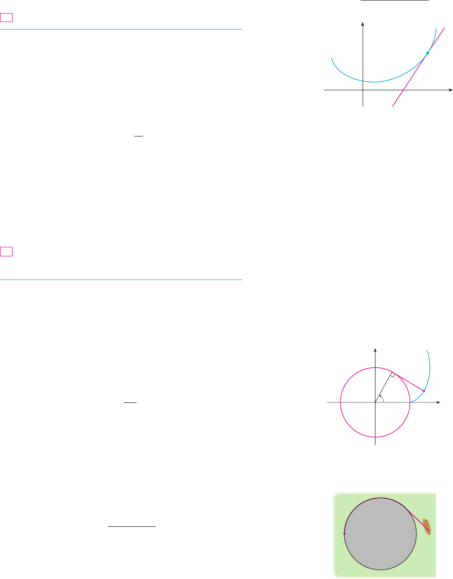
73. A string is wound around a circle and then unwound while

being held taut. The curve traced by the point at the end of

the string is called the involute of the circle. If the circle has

radius and center and the initial position of is ,

and if the parameter is chosen as in the ﬁgure, show

that parametric equations of the involute are

74. A cow is tied to a silo with radius by a rope just long

enough to reach the opposite side of the silo. Find the area

available for grazing by the cow.

y ! r "sin

cos

#x ! r"cos

sin

"r, 0#POr

! 1!rr

! 0

y ! 1 " cos

x !

" sin

"1, 1#y ! x

y!dx

(1 # "dy!dx#

)

3!2

xy ! f "x#x ! x

y ! f "x#

59–61 Find the exact area of the surface obtained by rotating the

given curve about the -axis.

59. , ,

60. , ,

, ,

;

62. Graph the curve

If this curve is rotated about the -axis, ﬁnd the area of the

resulting surface. (Use your graph to help ﬁnd the correct

parameter interval.)

63. If the curve

is rotated about the -axis, use your calculator to estimate the

area of the resulting surface to three decimal places.

64. If the arc of the curve in Exercise 50 is rotated about the

-axis, estimate the area of the resulting surface using Simp-

son’s Rule with .

65–66 Find the surface area generated by rotating the given

curve about the -axis.

, ,

66. , ,

67. If is continuous and for , show that the

parametric curve , , , can be put in

the form . [Hint: Show that exists.]

68. Use Formula 2 to derive Formula 7 from Formula 9.2.5 for

the case in which the curve can be represented in the form

, .

69. The curvature at a point of a curve is deﬁned as

where is the angle of inclination of the tangent line at ,

as shown in the ﬁgure. Thus the curvature is the absolute

value of the rate of change of with respect to arc length. It

can be regarded as a measure of the rate of change of direc-

tion of the curve at and will be studied in greater detail in

Chapter 14.

(a) For a parametric curve , , derive the

formula

where the dots indicate derivatives with respect to , so

. [Hint: Use and Formula 2

to ﬁnd . Then use the Chain Rule to ﬁnd .]d

!dsd

!dt

! tan

"dy!dx#x# ! dx!dt

x#y## " x##y#

(x#

# y#

)

3!2

y ! y"t#x ! x"t#

a + x + by ! F"x#

y ! F"x#

a + t + by ! t"t#x ! f "t#

a + t + bf $"t# " 0f $

0 + t + 1y ! 4e

t!2

x ! e

" t

0 + t + 5y ! 2t

x ! 3t

65.

n ! 4

1 + t + 2y ! t "

x ! t # t

y ! 2 sin

" sin 2

x ! 2 cos

" cos 2

0 +

!2y ! a sin

x ! a cos

61.

0 + t + 1y ! 3t

x ! 3t " t

0 + t + 1y ! t

x ! t

674

|| ||

CHAPTER 11 PARAMETRIC EQUATIONS AND POLAR COORDINATES

The Bézier curves are used in computer-aided design and are named after the French mathema-

tician Pierre Bézier (1910–1999), who worked in the automotive industry. A cubic Bézier curve

is determined by four control points, and , and is

deﬁned by the parametric equations

where . Notice that when we have and when we have

, so the curve starts at and ends at .

1. Graph the Bézier curve with control points , , , and

Then, on the same screen, graph the line segments , , and . (Exercise 31 in

Section 11.1 shows how to do this.) Notice that the middle control points and don’t lie

on the curve; the curve starts at , heads toward and without reaching them, and ends

2. From the graph in Problem 1, it appears that the tangent at passes through and the

tangent at passes through . Prove it.

3. Try to produce a Bézier curve with a loop by changing the second control point in

Problem 1.

4. Some laser printers use Bézier curves to represent letters and other symbols. Experiment

with control points until you ﬁnd a Bézier curve that gives a reasonable representation of the

letter C.

5. More complicated shapes can be represented by piecing together two or more Bézier curves.

Suppose the ﬁrst Bézier curve has control points and the second one has con-

trol points . If we want these two pieces to join together smoothly, then the

tangents at should match and so the points , , and all have to lie on this common

tangent line. Using this principle, ﬁnd control points for a pair of Bézier curves that repre-

sent the letter S.

, P

"40, 5#.P

"50, 42#P

"28, 48#P

"4, 1#

"x, y# ! "x

, y

t ! 1

"x, y# ! "x

, y

t ! 00 + t + 1

y ! y

"1 " t#

# 3y

t"1 " t#

# 3y

"1 " t# # y

x ! x

"1 " t#

# 3x

t"1 " t#

# 3x

"1 " t# # x

, y

#, P

, y

#, P

, y

SECTION 11.3 POLAR COORDINATES

|| ||

675

POLAR COORDINATES

A coordinate system represents a point in the plane by an ordered pair of numbers called

coordinates. Usually we use Cartesian coordinates, which are directed distances from two

perpendicular axes. Here we describe a coordinate system introduced by Newton, called

the polar coordinate system, which is more convenient for many purposes.

We choose a point in the plane that is called the pole (or origin) and is labeled . Then

we draw a ray (half-line) starting at called the polar axis. This axis is usually drawn hor-

izontally to the right and corresponds to the positive -axis in Cartesian coordinates.

If is any other point in the plane, let be the distance from to and let be the

angle (usually measured in radians) between the polar axis and the line as in Figure 1.

Then the point is represented by the ordered pair and , are called polar coordi-

nates of . We use the convention that an angle is positive if measured in the counter-

clockwise direction from the polar axis and negative in the clockwise direction. If ,

then and we agree that represents the pole for any value of .

"0,

#r ! 0

P ! O

r"r,

POrP

11.3

polar axis

P(r,¨ )

F I G U R E 1

;

ZIER CURVES

L A B O R A T O R Y

P R O J E C T

We extend the meaning of polar coordinates to the case in which is negative by

agreeing that, as in Figure 2, the points and lie on the same line through

and at the same distance from , but on opposite sides of . If , the point

lies in the same quadrant as ; if , it lies in the quadrant on the opposite side of the

pole. Notice that represents the same point as .

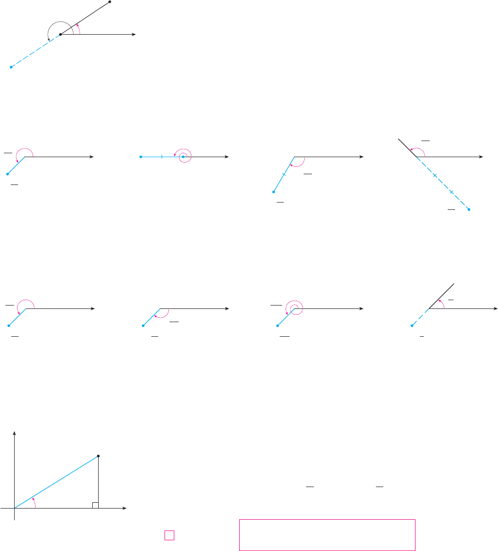
EXAMPLE 1 Plot the points whose polar coordinates are given.

(a) (b) (c) (d)

SOLUTION The points are plotted in Figure 3. In part (d) the point is located

three units from the pole in the fourth quadrant because the angle is in the second

quadrant and is negative.

In the Cartesian coordinate system every point has only one representation, but in the

polar coordinate system each point has many representations. For instance, the point

in Example 1(a) could be written as or or .

(See Figure 4.)

In fact, since a complete counterclockwise rotation is given by an angle 2 , the point

represented by polar coordinates is also represented by

where is any integer.

The connection between polar and Cartesian coordinates can be seen from Figure 5, in

which the pole corresponds to the origin and the polar axis coincides with the positive

-axis. If the point has Cartesian coordinates and polar coordinates , then,

from the ﬁgure, we have

and so

Although Equations 1 were deduced from Figure 5, which illustrates the case where

and , these equations are valid for all values of and (See the gen-

eral deﬁnition of and in Appendix D.)cos

sin

.r0

!2r $ 0

y ! r sin

x ! r cos

sin

cos

"r,

#"x, y#Px

"%r,

& "2n & 1#

#and"r,

& 2n

"r,

13π

”1, 



’

13π

3π

”1,_ 



’

3π

”1, ’

5π

F I G U R E 4

”_1,’

"%1,

!4#"1, 13

!4#"1, %3

!4#"1, 5

!4#

”_3, ’

3π

(2,3π)

3π

”1, ’

5π

F I G U R E 3

”2,_



’

2π

r ! %3

"%3, 3

!4#

"%3, 3

!4#"2, %2

!3#"2, 3

#"1, 5

!4#

"r,

#"%r,

"r,

#r $ 0OO

O"r,

#"%r,

r"r,

676

|| ||

CHAPTER 11 PARAMETRIC EQUATIONS AND POLAR COORDINATES

(_r,¨)

(r,¨)

¨+π

F I G U R E 2

P(r,¨)=P(x,y)

F I G U R E 5

Equations 1 allow us to ﬁnd the Cartesian coordinates of a point when the polar coor-

dinates are known. To ﬁnd and when and are known, we use the equations

which can be deduced from Equations 1 or simply read from Figure 5.

EXAMPLE 2 Convert the point from polar to Cartesian coordinates.

SOLUTION Since and , Equations 1 give

Therefore the point is in Cartesian coordinates.

EXAMPLE 3 Represent the point with Cartesian coordinates in terms of polar

coordinates.

SOLUTION If we choose to be positive, then Equations 2 give

Since the point lies in the fourth quadrant, we can choose or

. Thus one possible answer is ; another is .

Equations 2 do not uniquely determine when and are given because, as

increases through the interval , each value of occurs twice. Therefore, in

converting from Cartesian to polar coordinates, it’s not good enough just to ﬁnd and

that satisfy Equations 2. As in Example 3, we must choose so that the point lies in

the correct quadrant.

POLAR CURVES

The graph of a polar equation , or more generally , consists of all

points that have at least one polar representation whose coordinates satisfy the

equation.

EXAMPLE 4 What curve is represented by the polar equation ?

SOLUTION The curve consists of all points with . Since represents the distance

from the point to the pole, the curve represents the circle with center and radius

. In general, the equation represents a circle with center and radius . (See

Figure 6.) M

Or ! a2

Or ! 2

rr ! 2"r,

r ! 2

"r,

F"r,

# ! 0r ! f "

"r,

tan

0 '

NOTE

, 7

!4#

(

, %

)

! 7

! %

!4"1, %1#

tan

! %1

r !

& y

& "%1#

"1, %1#

(

)

y ! r sin

! 2 sin

! 2 !

x ! r cos

! 2 cos

! 2 !

! 1

!3r ! 2

"2,

!3#

tan

! x

& y

SECTION 11.3 POLAR COORDINATES

|| ||

677

F I G U R E 6

r=1

r=2

r=4

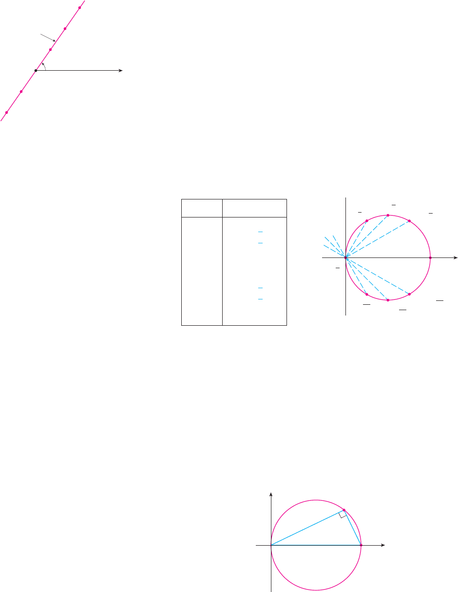
EXAMPLE 5 Sketch the polar curve .

SOLUTION This curve consists of all points such that the polar angle is 1 radian. It

is the straight line that passes through and makes an angle of 1 radian with the polar

axis (see Figure 7). Notice that the points on the line with are in the ﬁrst

quadrant, whereas those with are in the third quadrant. M

EXAMPLE 6

(a) Sketch the curve with polar equation .

(b) Find a Cartesian equation for this curve.

SOLUTION

(a) In Figure 8 we ﬁnd the values of for some convenient values of and plot the

corresponding points . Then we join these points to sketch the curve, which appears

to be a circle. We have used only values of between 0 and , since if we let increase

beyond , we obtain the same points again.

(b) To convert the given equation to a Cartesian equation we use Equations 1 and 2.

From we have , so the equation becomes ,

which gives

Completing the square, we obtain

which is an equation of a circle with center and radius 1. M

F I G U R E 9

"1, 0#

"x % 1#

& y

! 1

& y

% 2x ! 02x ! r

! x

& y

r ! 2x!rr ! 2 cos

cos

! x!rx ! r cos

F I G U R E 8

Table of values and

graph of r=2cos¨

(2,0)

”_1,’

2π

”0,’

”1,’

”œ

„

,’

”œ

„

,’

”_ œ

„

, ’

5π

”_ œ

„

, ’

3π

"r,

r ! 2 cos

r $ 0"r, 1#

"r,

! 1

678

|| ||

CHAPTER 11 PARAMETRIC EQUATIONS AND POLAR COORDINATES

(_1,1)

(_2,1)

(1,1)

(2,1)

(3,1)

¨=1

F I G U R E 7

0 2

r ! 2 cos

N Figure 9 shows a geometrical illustration

that the circle in Example 6 has the equation

. The angle is a right angle

(Why?) and so .r!2 ! cos

OPQr ! 2 cos

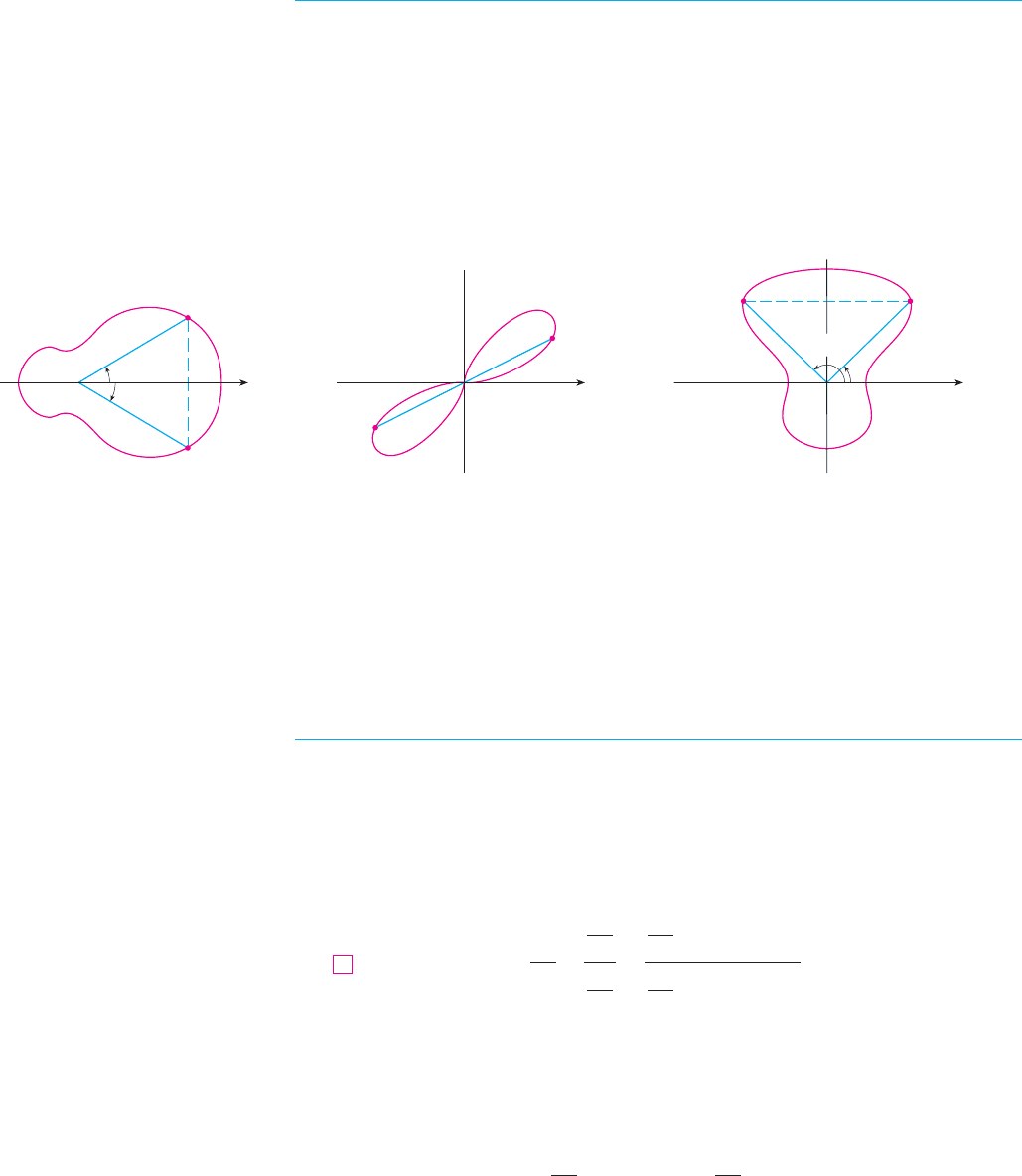
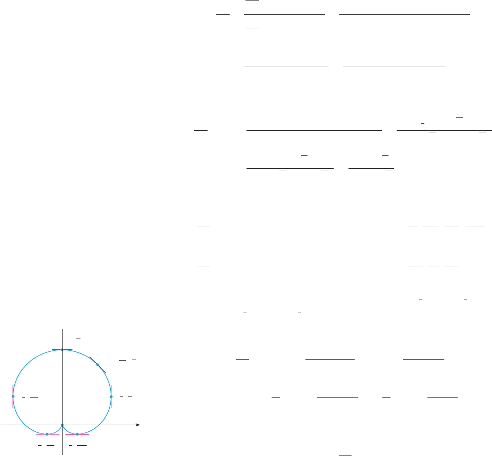
EXAMPLE 7 Sketch the curve .

SOLUTION Instead of plotting points as in Example 6, we ﬁrst sketch the graph of

in Cartesian coordinates in Figure 10 by shifting the sine curve up one

unit. This enables us to read at a glance the values of that correspond to increasing

values of . For instance, we see that as increases from 0 to , (the distance from )

increases from 1 to 2, so we sketch the corresponding part of the polar curve in Figure

11(a). As increases from to , Figure 10 shows that decreases from 2 to 1, so we

sketch the next part of the curve as in Figure 11(b). As increases from to ,

decreases from 1 to 0 as shown in part (c). Finally, as increases from to ,

increases from 0 to 1 as shown in part (d). If we let increase beyond or decrease

beyond 0, we would simply retrace our path. Putting together the parts of the curve from

Figure 11(a)–(d), we sketch the complete curve in part (e). It is called a cardioid,

because it’s shaped like a heart.

EXAMPLE 8 Sketch the curve .

SOLUTION As in Example 7, we ﬁrst sketch , , in Cartesian coordi-

nates in Figure 12. As increases from 0 to , Figure 12 shows that decreases from

1 to 0 and so we draw the corresponding portion of the polar curve in Figure 13 (indi-

cated by

). As increases from to , goes from 0 to . This means that the

distance from increases from 0 to 1, but instead of being in the ﬁrst quadrant this por-

tion of the polar curve (indicated by

) lies on the opposite side of the pole in the third

quadrant. The remainder of the curve is drawn in a similar fashion, with the arrows and

numbers indicating the order in which the portions are traced out. The resulting curve

has four loops and is called a four-leaved rose.

¨=0

¨=π

⑧

¨=

3π

¨=

F I G U R E 1 2

r=cos2¨ in Cartesian coordinates

F I G U R E 1 3

Four-leaved rose r=cos2¨

2ππ

5π

3π

7π

& ^

%1r

0 '

' 2

r ! cos 2

(a) (b) (c) (d) (e)

F I G U R E 1 1

Stages in sketching the cardioid r=1+sin¨

¨=π

¨=

¨=π

¨=

3π

¨=2π

¨=

3π

¨=0

¨=

r ! 1 & sin

SECTION 11.3 POLAR COORDINATES

|| ||

679

F I G U R E 1 0

r=1+sin¨ in Cartesian coordinates,

0¯¨¯2π

2π

3π

Module 11.3 helps you see how

polar curves are traced out by showing

animations similar to Figures 10–13.

TE C

SYMMETRY

When we sketch polar curves, it is sometimes helpful to take advantage of symmetry. The

following three rules are explained by Figure 14.

(a) If a polar equation is unchanged when is replaced by , the curve is symmetric

about the polar axis.

(b) If the equation is unchanged when is replaced by , or when is replaced by

, the curve is symmetric about the pole. (This means that the curve remains

unchanged if we rotate it through 180° about the origin.)

about the vertical line .

The curves sketched in Examples 6 and 8 are symmetric about the polar axis, since

. The curves in Examples 7 and 8 are symmetric about because

and . The four-leaved rose is also symmetric

about the pole. These symmetry properties could have been used in sketching the curves.

For instance, in Example 6 we need only have plotted points for and then

reﬂected about the polar axis to obtain the complete circle.

TANGENTS TO POLAR CURVES

To ﬁnd a tangent line to a polar curve , we regard as a parameter and write its

parametric equations as

Then, using the method for ﬁnding slopes of parametric curves (Equation 11.2.2) and the

Product Rule, we have

We locate horizontal tangents by ﬁnding the points where (provided that

). Likewise, we locate vertical tangents at the points where (pro-

vided that ).

Notice that if we are looking for tangent lines at the pole, then and Equation 3 sim-

pliﬁes to

" 0if

! tan

r ! 0

dy!d

" 0

dx!d

! 0dx!d

" 0

dy!d

! 0

sin

& r cos

cos

% r sin

y ! r sin

! f "

# sin

x ! r cos

! f "

# cos

r ! f "

0 '

cos 2"

# ! cos 2

sin"

# ! sin

!2cos"%

# ! cos

(r,¨)

(_r,¨)

(r,¨)

(r,_¨)

_¨

(a) (b) (c)

F I G U R E 1 4

(r,¨)(r,π-¨)

π-¨

%rr

680

|| ||

CHAPTER 11 PARAMETRIC EQUATIONS AND POLAR COORDINATES

For instance, in Example 8 we found that when or . This

means that the lines and (or and ) are tangent lines to

at the origin.

EXAMPLE 9

(a) For the cardioid of Example 7, ﬁnd the slope of the tangent line

when .

(b) Find the points on the cardioid where the tangent line is horizontal or vertical.

SOLUTION

Using Equation 3 with , we have

(a) The slope of the tangent at the point where is

(b) Observe that

Therefore there are horizontal tangents at the points , , and

vertical tangents at and . When , both and

are 0, so we must be careful. Using l’Hospital’s Rule, we have

By symmetry,

Thus there is a vertical tangent line at the pole (see Figure 15).

lim

!2#

! %(

! %

lim

!2#

%sin

cos

! (! %

lim

!2#

cos

1 & sin

lim

!2#

lim

!2#

1 & 2 sin

1 % 2 sin

lim

!2#

cos

1 & sin

dx!d

dy!d

! 3

(

, 5

)(

)

(

, 11

)(

, 7

)

"2,

!2#

when

! "1 & sin

#"1 % 2 sin

# ! 0

when

! cos

"1 & 2 sin

# ! 0

1 &

%1 %

! %1!

1 &

(

2 &

)(

1 %

)

(

1 &

)

(

1 &

)(

1 %

)

cos"

!3#"1 & 2 sin"

!3##

"1 & sin"

!3##"1 % 2 sin"

!3##

cos

"1 & 2 sin

1 % 2 sin

% sin

cos

"1 & 2 sin

"1 & sin

#"1 % 2 sin

sin

& r cos

cos

% r sin

cos

sin

& "1 & sin

# cos

cos

% "1 & sin

# sin

r ! 1 & sin

r ! cos 2

y ! %xy ! x

! 3

!4r ! cos 2

! 0

SECTION 11.3 POLAR COORDINATES

|| ||

681

5π

”, ’

7π

”, ’

”, ’

11π

” , ’

(0,0)

m=_1

”1+ ,’

„3

”2,’

F I G U R E 1 5

Tangent lines for r=1+sin¨

Openmirrors.com