Szilas A.P. Production and transport of oil and gas, Gathering and Transportation
Подождите немного. Документ загружается.

3
10
Loop
Pipeleg
X.
PIPELINE TRANSPORTATION
OF
NATURAL GAS
Table
4
m
3
0.307
I
01541
0.1541
o.2w
0.1541
0.1023
0.1023
0.
I023
01023
0.1541
0.1023
0.
I023
01541
0.1541
0307
1
0.205
I
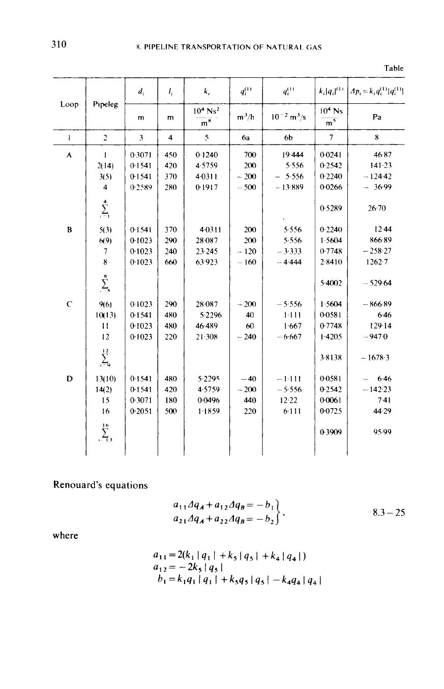
Renouard's equations
where
4
450
420
370
2x0
~
370
290
240
660
290
4x0
4x0
220
480
I
no
420
5m
5
0.
I
240
4.5759
4.03
I
I
0.1917
4.03
I I
2x.0~7
23.245
63.923
2x087
5.2296
464R9
2
I
,3ox
5.2295
4.5759
0.0496
1.i~
4:"
mJ/h
6d
700
200
-
200
~~
500
200
200
-
120
~~
160
-
200
40
60
-
240
-
40
--
200
440
220
4!l'
6b
19.444
5-556
-
5.556
-
1~x9
5.556
5.556
-
3.333
-
4.444
~
5.556
1-1
I
I
1.667
~
6667
-1.111
-
5.556
12.22
6.1
11
7
0.024
1
0.2542
0.2240
0.0266
-
0.5289
0.2240
1
,5604
2.X410
0.7748
5.4002
1.5604
0.058
I
0.774~
1.4205
3.8
I
3x
0.058
I
0.2542
0.006
I
0.0725
0.3909
Pa
n
46.R7
141.23
~-
124.42
-
36.99
2670
12.44
-
258.27
~66.89
1262.7
~~
529-64
-
866.R9
646
129.14
~-
947.0
-
1678.3
-
6.46
-
142.23
7.4
I
44.29
95.99
8.3
-
25
8.3.
STEADY-STATE
FLOW
IN
PIPELINE
SYSTEMS
31
1
8.3
~
3
__
...
9!2'
PI, PII,
m3
10
~
s
m3/h
ra
ra
9
10
1
la
Ilb
12
13
14
19.192
4.076
-
14.141
-
6.298
6298
3.846
-
2.843
-
3.954
-
3.846
2,083
3,867
~
4.466
-
2.083
-
4.076
13.450
7.339
...
...
...
...
...
...
...
...
...
...
...
...
...
...
20.960
4.532
-
5.486
~
12.373
5.486
-
1
.xnx
4.353
-
2.999
-4.353
I
.220
4.315
-
4.018
-
1.220
-4.532
14.762
8.65
1
754.6
163.2
-
197.5
-
445.4
197.5
156-7
-
68.0
-
108.0
-
156.7
43.9
155.3
144.6
-
43.9
-
163.2
53
I
.4
31
1.4
54.47
-
12
I
.30
~
29.35
~
2.20
121.30
532. I4
~
574.75
~
4.12
93.98
~ 82.81
-
532.14
1.79
865.76
-
343.98
-~
2.58
-
7.7$
10.8
I
-
93.98
88.74
-
2.22
3300
3246
3152
3273
3273
3152
2619
2702
2619
3152
3144
2278
3144
3152
3246
3235
3246
3152
3273
3302
3152
2619
2702
3277
3152
3144
2622
2278
3152
'
3246
3235
3146
-
0.252
0.490
2.200
1.228
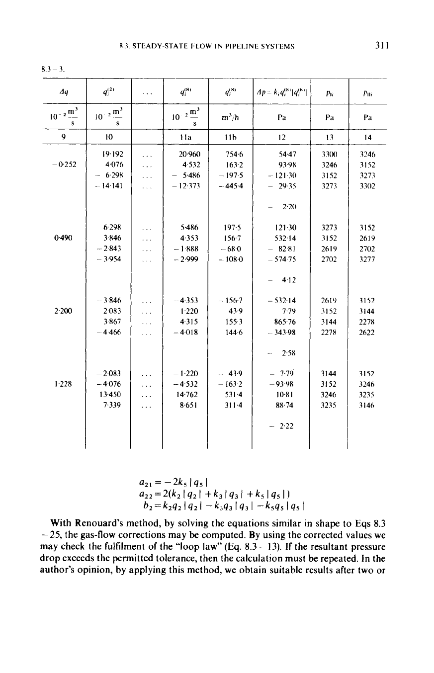
a21
=
-2k
145
I
a22=2@2
I42
I
+k3
I
q3
I
+k
I
45
I)
b2
=k242
I
42
I
-443
I43
I
-A545
145
I
With Renouard's method, by solving the equations similar in shape
to
Eqs 8.3
-25, the gas-flow corrections may
be
computed. By using the corrected values we
may check the fulfilment
of
the "loop law"
(Eq.
8.3-
13). If the resultant pressure
drop exceeds the permitted tolerance, then the calculati~n must be repeated. In the
author's opinion, by applying this method, we obtain suitable results after two
or
312
8. PIPELINE TRANSPORTATION
OF
NATURAL GAS
three iterations even in the case,
if
the starting values have significantly differed from
the proper values.
Stoner’s method for solving looped-networks is based on the node continuity
equation (Stoner
1970).
It has the advantage that, whereas the
Cross
method can be
used to establish throughput and pressure maps
of
the network only, the Stoner
method will furnish any parameter (pipe size in a leg, compressor horsepower
required, number of storage wells, size of pressure-reducing choke, etc.) of the
complex system. It is, however, significantly more complicated than the previously
mentioned methods, and
it
requires much more computer time.
-
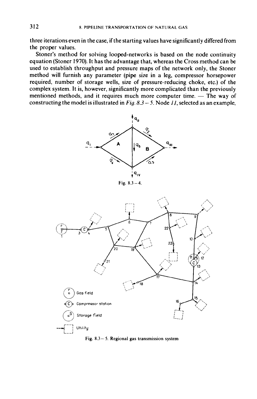
The way
of
constructing the model is illustrated in
Fig.
8.3
-5.
Node
1
I,
selected as an example,
;ql”
Fig.
8.3
-
4.
a
Gas
fleld
c@
Compressor
station
Storage field
16
A/-
--ir--;
utility
L--J
Fig.
8.3
-
5.
Regional gas transmission
system
X.3.
STEADY-STATE
FLOW
IN
PIPELINE SYSTEMS
313
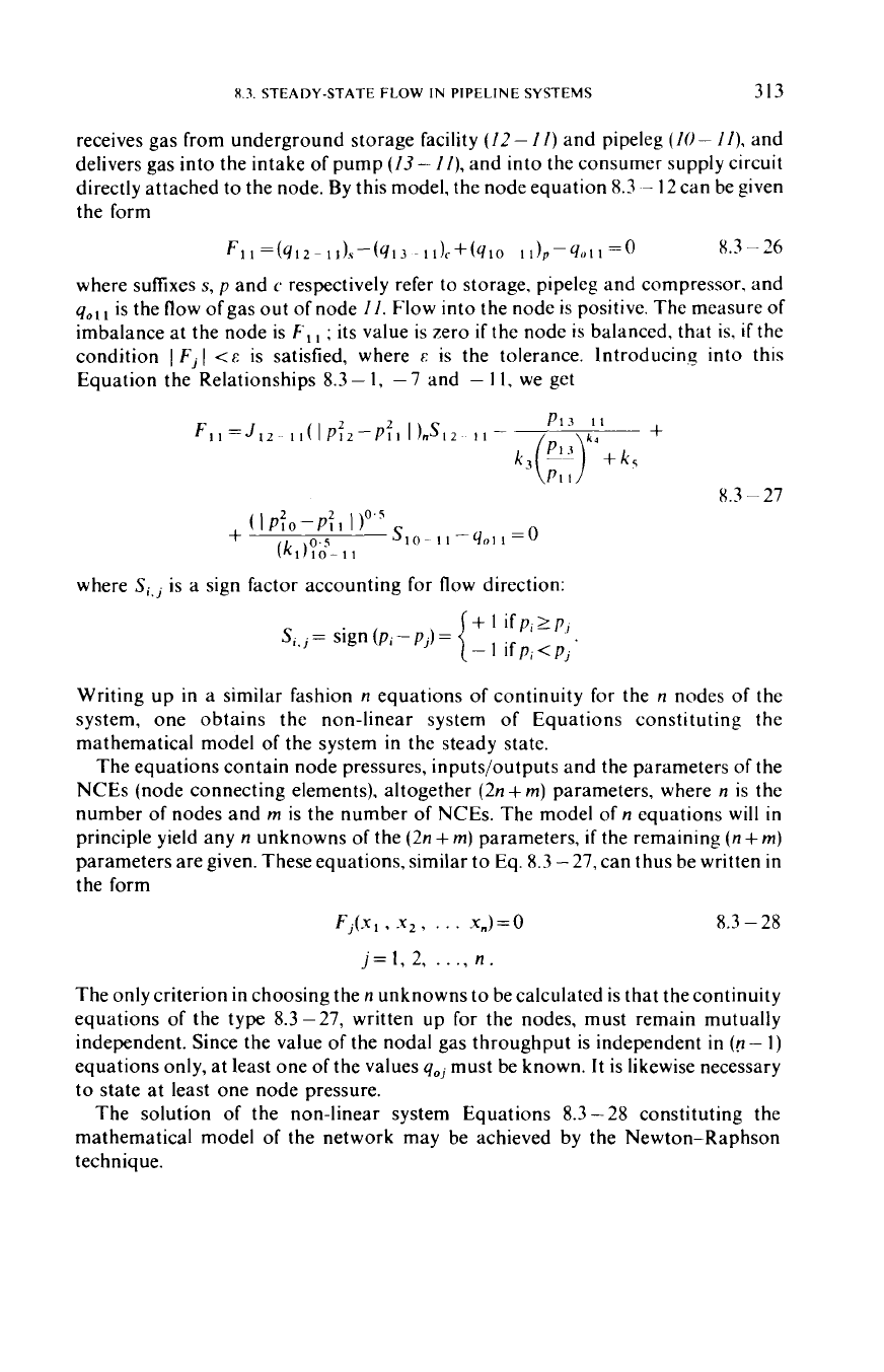
receives gas from underground storage facility
(12
-
1
/)
and pipeleg
(10
-
1
I),
and
delivers gas into the intake of pump
(13-
/I),
and into the consumer supply circuit
directly attached
to
the node. By this model, the node equation
8.3
-
12
can be given
the form
F11=(q12-11)\-(413
ll)c+(qlO
Il)p-qoIl=o
8.3
-
26
where suffixes
s,
p
and
L'
respectively refer to storage. pipeleg and compressor, and
yo,
is the flow ofgas out of node
//.
Flow into the node is positive. The measure
of
imbalance at the node is
F',
I
;
its value is
zero
if
the node is balanced, that is,
if
the
condition
IF,
1
<E
is satisfied, where
E
is the tolerance. Introducing into this
Equation the Relationships
8.3-
I,
-7
and
-
I
I.
we get
X.3
-
27
where
Si.j
is a sign factor accounting for
flow
direction:
Writing up in a similar fashion
n
equations of continuity for the
n
nodes of the
system, one obtains the non-linear system of Equations constituting the
mathematical model of the system in the steady state.
The equations contain node pressures, inputs/outputs and the parameters of the
NCEs (node connecting elements). altogether
(2n
+
m)
parameters, where
n
is the
number of nodes and
m
is the number of
NCEs.
The model
of
n
equations
will
in
principle yield any
n
unknowns of the
(2n
+
m)
parameters,
if
the remaining
(n
+
m)
parameters are given. These equations, similar to Eq.
8.3
-
27,
can thus be written
in
the form
Fj(x
,
.Y2
,
. . .
x,)
=
0
8.3
-
28
j=l,2,
...,
n.
The only criterion in choosing then unknowns to becalculated is that thecontinuity
equations of the type
8.3
-
27,
written up for the nodes, must remain mutually
independent. Since the value of the nodal gas throughput is independent in
(g
-
1)
equations only, at least one
of
the values
yo,
must be known.
It
is likewise necessary
to state at least one node pressure.
The solution of the non-linear system Equations
8.3
-
28
constituting the
mathematical model
of
the network may be achieved by the Newton-Raphson
technique.

314
8.
PIPELINE TRANSPORTATION
OF
NATURAL GAS
Fig.
8.3
-6.
Pseudo-isobar curves
of
a
low
pressure
gas
distribution system
(I)
Fig.
8.3
-
7.
Psuedo-isobar curves
of
a
low
pressure
gas
distribution system
(11)
X.4.
TRANSIENT
FLOW
IN
PIPELINE
SYSTEMS
315
Stoner (1970,
1971),
in a development of the above method, gave a procedure for
determining the ‘sensitivity’ of the system
in
steady-state operation. The purpose of
the calculation is in this case to find out
in
what way some change(s) in some
parameter(s)
of
the system affect the remaining parameters. For instance, what
changes
in
input pressures and flow rates,
or
compressor horsepower, are to be
effected
in
order to satisfy a changed consumer demand?
The pressure distribution of the steady state flow
in
the gas networks is well
represented by the pseudo-isobar map.
A
given isobar curve connects the points of
equal pressure
in
the different pipelines of the network. They are called pseudo-
curves because the pressure lines, at areas outside the pipelines, have no physical
meaning. The pseudo-isobar maps may be used for the analysis of both high
pressure looped systems (Patsch
et
af.
1974),
and low-pressure looped gas-
distributing systems (Csete and
Soos
1974). In
Fig.
8.3-6
the pipelines
(full
line),
and the pseudo-isobars (dashed line) of a low-pressure gas-distributing system are
shown.
It
can be seen that first of all in field
A
the pseudo-isobar lines are “dense”,
the pressure drop is significant.
If
to this gas network the pipeline
in
Fig.
8.3-
7,
marked
with
thick dashed line, is fitted, then the pressure drop, in considerable part
of the pipe network is reduced more advantageous and this circumstance may
justify the building
of
the new line.
8.4.
Transient
flow
in pipeline systems
The flow
is
transient
in
every pressure level gas transmission network, but its
simulation has a practical significance in high pressure system design only (see the
introduction of the Section 8.3). One of the aims of transient flow simulation is the
numerical mapping
of
the flow characteristics of imagined or planned situation (eg
the determination of maximum throughput capacity at given bounds,
or
the effect of
a leak
in
a given pipeline leg). For the dispatch center
it
is a great help to incorporate
a computer being able to evaluate unexpected situations and to suggest alternatives
for solution by aid ofa transient flow program (Gibbon and Walker 1978). Another
task can be. to show, what
will
be the effect of a planned modification (e.g. of
building a pipeline leg, or compressor station). Simpler problems can be solved
approximately by use of a steady state model too. They do not take into account,
however, the change of the mobile gas caused by the variation of the system pressure
and hence the excess gas flowing through the regulator station from the high
pressure system into the gas distribution network simultaneously with the pressure
drop. By the transient model
it
becomes possible to know accurately the transport
capacity of the system and to utilize
it.
As
a result. sometime costs
of
a new
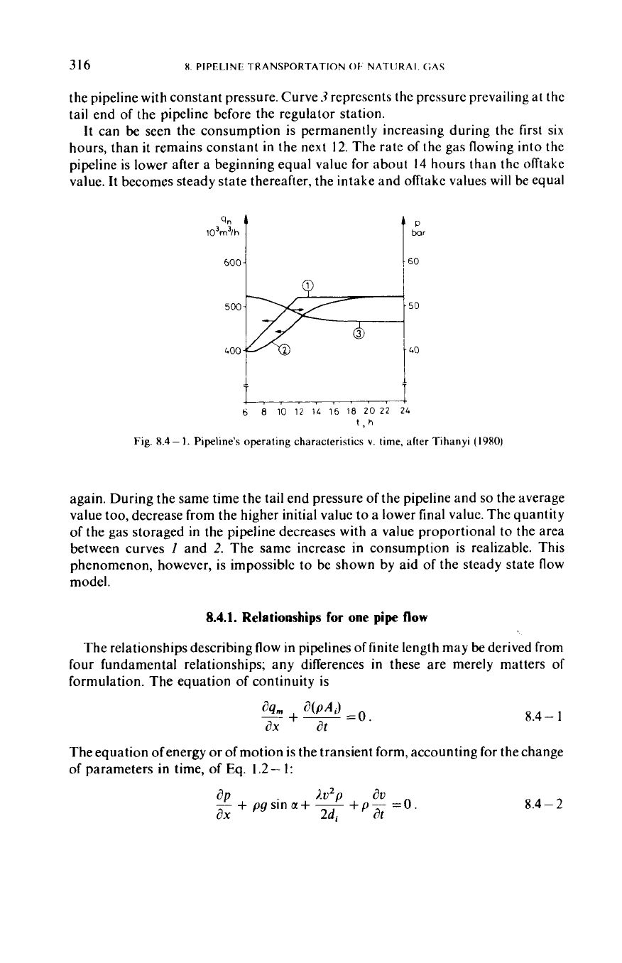
investment increasing capacity may be spared. As an example
Fig.
8.4
-
I
after
Tihanyi (1980) shows curves characterizing the transient operation
of
a pipeline of
200
km length and 0.8 m diameter. Curve
I
represents the gas stream flowing out of
the pipeline (this will be the consumed gas), curve
2
models the gas rate injected into
316
X.
PIPELINE TRANSPORTATION
OF
NATIJRAI.
GAS
the pipeline
with
constant pressure. Curve
3
represents the pressure prevailing at the
tail end
of
the pipeline before the regulator station.
It
can
be
seen the consumption is permanently increasing during the first six
hours, than
it
remains constant
in
the next
12.
The rate
of
the gas flowing into thc
pipeline is lower after a beginning equal value for about
14
hours than the offtake
value.
It
becomes steady state thereafter, the intake and offtake values will be equal
1
T
1
T
LA
6
8
10
12
1L
16
18
20
22
24
',h
Fig.
8.4-
I.
Pipeline's
operating characteristics
v.
time, after Tihanyi
(1980)
again. During the same time the tail end pressure of the pipeline and
so
the average
value too, decrease from the higher initial value to a lower final value. The quantity
of the gas storaged in the pipeline decreases with a value proportional to the area
between curves
I
and
2.
The same increase
in
consumption is realizable. This
phenomenon, however, is impossible to be shown by aid of the steady state flow
model.
8.4.1.
Relationships
for
one
pipe
flow
The relationships describing flow in pipelines
of
finite length may
be
derived from
four fundamental relationships; any differences in these are merely matters of
formulation. The equation
of
continuity is
8.4-
1
The equation
of
energy or
of
motion is the transient form, accounting for the change
of parameters in time, of
Eq.
1.2
-
1:
dVzp
ao
+p-
=o.
aP
-
+
pgsina+
~
ax
2di
at
8.4
-
2
8.4.
TRANSIENT
FLOW
IN
PIPELINE
SYSTEMS
317
The equation of state for a gas flow regarded as isothermal is, by Eq.
8.1
-
1
The fourth fundamental relationship
z
=
f(P)T
3
has several solutions employed
in
practice, one of which is Eq.
8.
I
-
9.
If
z
is replaced
by its average value and considered constant, then the number of fundamental
equations reduces to three, and Eq.
8.1
-
1
may be written in the simpler form
-
P
=B2,
P
where
B
is the isothermic speed of sound. Eqs
8.4-
1
and
8.4- 3
imply
where mass flow is
q
=pAiv= Aiv.
B2
m
By Eqs
8.4-2, 8.4-3
and the above definition of
qm,
8.4
-
3
8.4
-
4
8.4
-
5
Equations
8.4-4
and
-5
constitute a system of non-linear partial differential
equations; then, on the assumption that ?=constant, describe transient flow
in
the
pipeline system.
In the approach
to
the numerical solution of the system
of
partial differential
Equations
8.4-4
and
8.4-
5,
the system is transformed into a system of algebraic
equations using the method of finite differences. This algebraic system is capable of
solution.
For
the transformation, the method ofcentral finite differences can
be
used
to advantage. It consists in essence of replacing the function, continuous in the
interval under investigation, by a chord extending across a finite domain of the
independent variable. The slope
of
said chord
is
approximately equal to the slope of
the tangent to the curve at the middle
of
the domain.
It
is subsequently simple to
calculate numerically the derivative
of
the curve.
For
solving the system of differential equations, literature (e.g. Zielke
1971)
usually cites three methods:
the implicit method, the explicit method and the method
of
characteristics.
A
common trait to the three methods is that calculation proceeds
step by step, deriving pressures and flow rates prevailing at various points of the
pipeline at the instant
t
+
At
on the basis of the known distribution of pressures and
318
X
PIPELINE
TRANSPORTATION
Of
U;\TIIKAI
(i.\S
flow rates at the instant
t.
The differences are as follows.
-
In
the explicit method,
the partial differential equations are transformed into algebraic equations.
so
that
the unknown pressures and flow rates at the instant
t+At
depend only on the
known pressures and
flow
rates
of
the preceding time
step.
which perrnits
us
to find
their values one by one solving the individual equations for them.
~
In
the implicit
method, a system of algebraic equations results, which contains the
unknown
pressures and flow rates at the instant
[+At
at the neighbouring points
of
the
pipeline
so
as
to
be made available only by the solution
of
the entire simullnneous
set of equations. The system of equations furnished by the transformation may,
in
both cases, be either linear or not. There is the fundamental difference that. whereas
in
the explicit system the time step is limited
for
reasons of stability. the only
consideration that limits the time step
in
the implicit method is the accurucv
required, but steps are usually significantly longer than what is admissiblc
in
thc
explicit method.
-~
The method of characteristics is essentially an explicit method
whose essence is
to
seek
in
the
[.Y,
t]
plane such directions along which the partial
differential equation can be reduced
to
a common differential equation.
This
latter
can be solved numerically by the method of finite differences. The
time
c!ep
is
rather
restricted also
in
this method.
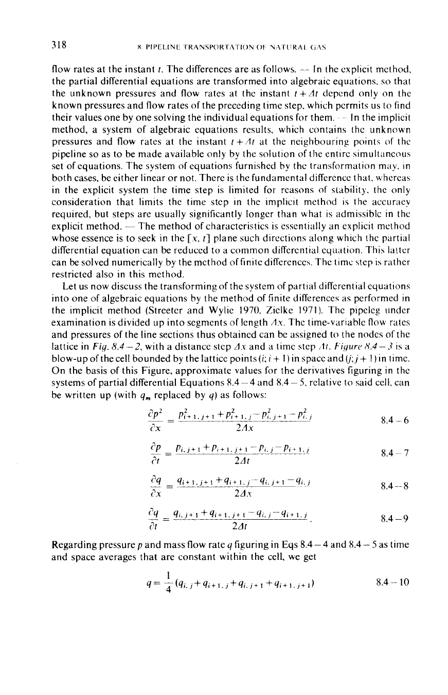
Let us now discuss the transforming
of
the system of partial differential equations
into one of algebraic equations by the method of finite differences as performed
in
the implicit method (Streeter and Wylie 1970. Zielke 1971). The
pipeleg
under
examination is divided up into segments
of
length
Au.
The time-variable
flow
rates
and pressures
of
the line sections thus obtained can be assigned to the nodes
of
the
lattice in
Fig.
8.4
-2,
with a distance step
Au
and a time step
,It.
F'icqure
8.4-3
is a
blow-upofthecell bounded by thelattice points(i;i+
1)in
spaceandu;,j+
I)in
time.
On the basis
of
this Figure, approximate values
for
the derivatives figuring
in
the
systems of partial differential Equations 8.4-4 and 8.4-
5,
relative to said cell. can
be written up
(with
qm
replaced by
4)
as follows:
8.4
-
6
8.4
-
8
8.4
-
9
Regarding pressure
p
and mass flow rate
y
figuring
in
Eqs 8.4
-
4 and 8.4
-
5
as time
and space averages that are constant within the cell, we get
8.4-
10
1
4
4=
-(4i.
j+
4i+
1.
j+4i,
j+
I
+Yi+
I.
,+
I)

8.4.
TRANSIENT
FLOW
IN PIPELINE
SYSTEMS
319
I
x
1-1
I
i+l
i+2
Fig.
8.4
-
2.
I
J+’
I
I
-
1 i+t
Fig.
8.4-3.
1
4
P=
-(Pi,j+Pi+1,j+Pi,j+i+Pi+1.j+i)
8.4-
11
Resubstituting
Eqs
8.4
-
6
to
8.4
-
1
1
into
Eqs
8.4- 4 and 8.4
-
5,
and rearranging,
we
have a system
of
non-linear algebraic equations:
1
At
F1=
-
(Pi,
j+
1
+Pi+
1,
j+
1
-Pi.
j-Pi
+
1.
j)
+