Tong W. Wind Power Generation and Wind Turbine Design

Подождите немного. Документ загружается.

Wind Turbine Acoustics 165

5 Wind turbine noise measurements

There are two main categories of measurements related to wind turbine acoustics:

on-site and wind-tunnel measurements. The ﬁ rst group gives more realistic data

since it is applied for a whole wind turbine and gives directly the noise generated

by it. The major drawbacks of the on-site measurements are the difﬁ culty to install

the instrumentation and the impossibility of prescribing desired ﬂ ow conditions.

This leads also to a limited repeatability of the measurements. Wind-tunnel mea-

surements offer more control, but they have a limited size. As a consequence,

the models have to be scaled down and sometimes only parts of the wind turbine

can be studied. The scaling of the models is not straightforward, not all the non-

dimensional parameters can be preserved. Also, the background noise from the

wind tunnel is difﬁ cult to subtract from the measurements. A good review of the

measurement methods applicable for wind turbine noise is presented in [ 4 ].

5.1 On-site measurements

5.1.1 Ground board

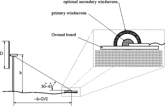
The ground board consists of a ﬂ at, acoustically hard plate with a microphone

mounted horizontally, at the center of the plate [ 4 ]. The microphone has to be directed

towards the turbine tower and is covered by a wind screen (see Fig. 11 ). The major

advantage of using a ground board is that it diminishes the wind-induced noise and

that the reﬂ ections from the ground are independent from the site. To remove the

effect of reﬂ ections 6 dB is subtracted from the measured spectra at all frequencies.

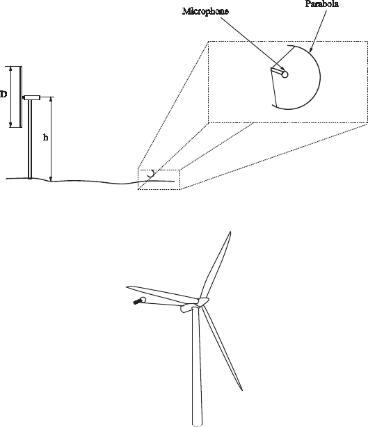
5.1.2 Acoustic parabola

Acoustic parabolas (see Fig. 12 ) reﬂ ect and focus the acoustic waves in their focal

point where a microphone registers the signal. The ampliﬁ cation depends on the

Figure 11: Ground board used for noise measurements (after [ 4 ]).

166 Wind Power Generation and Wind Turbine Design

angle of incidence, it ampliﬁ es more the noise coming from the direction where

the parabola is aimed to.

In this way noise coming from a certain part of the wind turbine can be local-

ized. If one is interested in the noise coming from a certain part of the rotating

blades (e.g. tip region), the measured signal has to be windowed to post process

only the data corresponding to the passage of the blade over the measurement spot.

The ampliﬁ cation depends also on the wavelength of the acoustic waves, large

wavelengths compared to the size of the parabola reduces the spatial accuracy.

5.1.3 Proximity microphone

Ground boards and acoustic parabolas are used far from the wind turbine. Prox-

imity microphones (see Fig. 13 ) are installed close to the noise sources, either on

the blades themselves or close to the blades on ﬁ xed devices. The disadvantage

of mounting the proximity microphones directly on the blades is that it will be

exposed to higher speeds of the air ﬂ ow resulting in higher wind-induced noise.

If the microphone is not co-rotating with the blade a time-windowing technique

has to be used to collect data only when the noise sources are in the vicinity of the

Figure 12: Acoustic parabola used for noise measurements.

Figure 13: Proximity microphone used for noise measurements.

Wind Turbine Acoustics 167

microphone. The spatial accuracy of the proximity microphones depends on the

distance from the source, but, unlike acoustic parabolas, is independent of the

acoustic wavelength.

5.1.4 Acoustic antenna

Acoustic antennas are composed by a set of microphones in a row or in a matrix

which can be mounted on a ground plate or in the proximity of the wind turbine.

By computing correlations of the signals provided by different microphones, the

location of the acoustic sources can be determined.

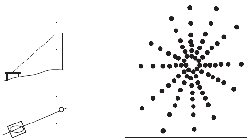
Oerlemans et al. [ 16 ] used for example an array of 148 microphones mounted

on a board of 15 m × 18 m. The array had an elliptic shape to account for the cir-

cular motion of the blades and for the tilted angle of the board (see Fig. 14 ). Cross-

correlating the microphones data made possible to determine the distribution of

the noise sources in the rotor plane and along the rotor blades (individually for the

three blades). It was observed that most of the noise sources are located on the

right-hand side of the rotor plane, indicating that most of the noise is generated

during the downward motion of the blades. Furthermore, the contribution of the

hub was also clearly visible.

5.2 Wind-tunnel measurements

Wind tunnels have the advantage of providing better controllable ﬂ ow conditions

and thus are preferred for systematic studies. Due to their size limitations, how-

ever, wind tunnels are limited to downscaled model studies. The large-scale facil-

ity at the National Renewable Energy Laboratory in the USA is equipped with

a wind tunnel with a measurement cross section of 24.4 × 36.6 m

which made

possible to carry out ﬂ ow measurements on a full-scale (10 m rotor diameter) wind

turbine [ 17 ]. The wind tunnel, however, is not anechoic, thus is not well suited for

acoustic measurements.

Figure 14: Sketch of the board position (left) and the arrangement of the micro-

phones on the board (right) (after [ 16 ]).

168 Wind Power Generation and Wind Turbine Design

Brooks et al. [ 18 ] measured the ﬂ ow and the acoustic pressure around a set of

NACA 0012 airfoils with different chord lengths in an anechoic chamber. Eight

microphones have been used for the noise measurements. Based on the measure-

ment data, semi-empirical models have been developed to predict airfoil self-noise

(see Section 6.2).

In Europe there are two anechoic wind tunnels at the University of Oldenburg

and at the National Aerospace Laboratory (NRL) in the Netherlands [ 4 ]. These

facilities have been used also for the study of the airfoil self-noise, as well as for

the study of the noise due to turbulent inﬂ ow.

The major drawback of wind-tunnel measurements is the self-noise of the wind

tunnel itself. The errors due to the background noise can be reduced for rotating

sources by using tracking methods. For stationary sources (e.g. airfoil cross sec-

tions) the error due to the background noise can be reduced by using multiple

microphones and cross-correlating the signals at different observer positions.

Fujii et al. [ 19 ] studied the noise generated by the interaction of the rotor blades

with the wakes of wind turbine towers. Towers with circular, elliptical and square

cross sections have been considered. Their measurements showed that the tower

with a slender elliptic cross section was the quietest, the loudest being the one with

the square cross section.

6 Noise prediction

The solution of the compressible Navier-Stokes equations includes inherently also

the generation and propagation of the acoustic pressure waves. This direct compu-

tational approach, however, involves several drawbacks, which make it applicable

only for relatively simple cases and to small Reynolds numbers [20 − 22]. One issue

is the small magnitude of the acoustic quantities (acoustic pressure and density

ﬂ uctuations) as compared to the hydrodynamic quantities of the ﬂ ow. The low-

amplitude acoustic ﬂ uctuations require discretization schemes with high accu-

racy which are computationally demanding. Also, the timesteps are limited by the

sound speed and not the convection speed as it is the case of incompressible ﬂ ow

simulations. As a result, there was a need to develop aeroacoustic models.

Lighthill [ 23 ] was the ﬁ rst to derive a model for aerodynamically generated

sound. By rearranging the continuity and momentum equations he obtained the

following non-homogeneous wave equation for the acoustic density:

()

ii i j

xx xx

∂

∂∂

−=

∂∂ ∂∂

∂

(10 )

where r ′ = r − r

is the acoustic density ﬂ uctuation deﬁ ned as the departure from

ambient conditions, and c

is the sound speed in the undisturbed ambient medium.

In the derivation of eqn ( 10 ) it was assumed that the ambient conditions are con-

stant and viscosity effects have been neglected. Equation ( 10 ) is called the Light-

hill analogy and describes the propagation (left-hand side, LHS) and generation

(right-hand side, RHS) of sound by the ﬂ uid ﬂ ow. The term on the RHS is the

Wind Turbine Acoustics 169

second derivative of the Lighthill stress tensor, T

= r u

, which acts as a source

of quadrupole type.

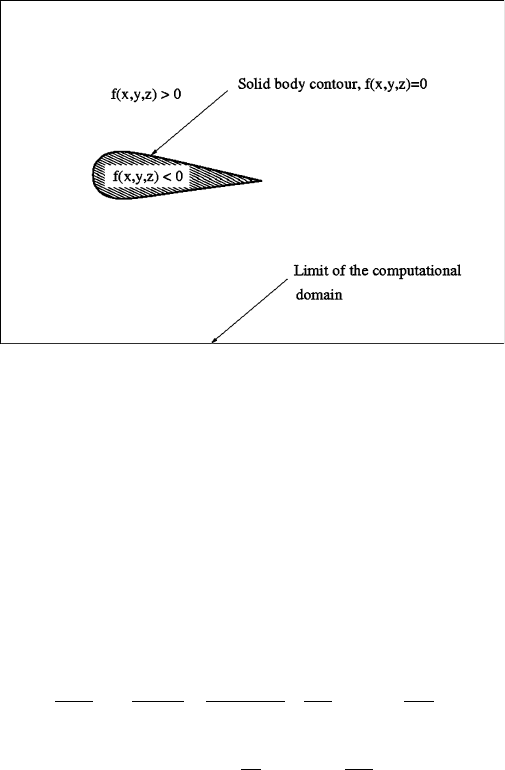
Lighthill's analogy does not take into account the noise generated by solid

surfaces. To remedy this deﬁ ciency, Ffowcs Williams and Hawkings (cited in

[ 24 ]) extended Lighthill’s analogy by representing a solid object by a sur-

face S deﬁ ned as f ( t,x,y,z ) = 0 (see Fig. 15 ) and extending the ﬂ uid motion

also into the object domain but restricting the velocity to the speed of the

object itself. Using the generalized function theory the following equation has

been derived:

()

ii i j i j

cpf

xx xx x x

⎛⎞

∂

∂∂ ∂ ∂

−= −

⎜⎟

∂∂ ∂∂ ∂ ∂

∂

⎝⎠

⎛⎞

∂∂

⎜⎟

∂∂

⎝⎠

(11 )

The ﬁ rst term on the right-hand side is identical to the RHS of eqn ( 10 ) and is

the Lighthill stress tensor. The second term on the RHS is proportional to the stress

tensor p

, reﬂ ecting the force which the object exerts on the ﬂ uid and it has a

dipole character. The third term on the RHS is a monopole term and is proportional

to the acceleration of the ﬂ uid by the non-stationary solid surface.

Based on these theoretical models, researchers deduced semi-empirical models

used for the prediction of the noise generated by non-rotating and rotating air-

foils. The ﬁ rst models were developed to predict the noise generated by airplane

wings and helicopter rotors. Later, these models were adapted for wind turbine

applications. With the increase of the available computational power and evolu-

tion of the aeroacoustic theory more and more complex models were developed

Figure 15: The value of the shape function in the solid and ﬂ uid regions.

170 Wind Power Generation and Wind Turbine Design

during the years. Lowson (cited in [ 4 ]) divided the prediction models in three

categories:

The Category I models predict the global emitted noise as a function of main •

wind turbine parameters, like rated power, rotor diameter, blade area, tip

speed, etc.

The Category II models are semi-empirical relationships which predict the total •

sound pressure level and spectral shape taking into account the various noise

generation mechanisms.

The Category III models are based on a detailed description of the rotor geometry •

and aerodynamics and give detailed information about the acoustic ﬁ eld.

6.1 Category I models

These models are the simplest ones. Based on simple algebraic relations they

predict the emitted sound power level as functions of the wind turbine main

parameters. Table 1 lists the category I models as it is summarized by Wagner

et al. [ 4 ]. In Table 1 L

is the total A-weighted sound power level, P

the rated

power of the turbine, D the rotor diameter, L

the A-weighted sound pressure

level at a monitoring point located at a distance of r

from the tower base, V

tip

the

tip speed, n

the number of the blades, A

the blade area, A

the rotor area, C

the

axial force coefﬁ cient, r the hub − observer distance. C

are empirical parameters

having different values in different references.

These Category I models are simple and fast, however they are by far not univer-

sal. As a consequence, these models were rapidly outranked by the computationally

not much more expensive, but more accurate Category II models.

6.2 Category II models

The models belonging to this category are semi-empirical and consist of a set

of models for the noise generation mechanisms listed in Section 4.1.2. Based on

Lighthill's and Ffowcs Williams − Hawkings theory and experimental measurements

Table 1: Category I models [ 4 ].

No. Model

WA 10 WT

10 log 50LP=+

WA 10

22 log 72LD=+

pA 1 10 tip 2 10 b 3 10 T 4 10 5 10 6

log log log log log

LC VC n C CC C DC

⎛⎞

=+ ++−−

⎜⎟

⎝⎠

Wind Turbine Acoustics 171

algebraic relationships are deduced to model both the emitted sound power level

and sound spectrum. There are a multitude of models in the literature for each

noise generation mechanism, in the followings the most widespread models

being presented.

6.2.1 Trailing edge noise

Grosvelds model (cited in [ 4 ]) is based on a frozen turbulent pattern convected

downstream over the trailing edge and predicts the A-weighted sound pressure

level as:

pA 10 b

10 log ( )

LnKfC

⎛⎞

=++

⎜⎟

⎝⎠

(12)

The shape of the spectrum is given by

4 1.5

max max

( ) 10log 0.5

St St

−

⎧⎫

⎡⎤

⎛⎞⎛⎞

⎪⎪

⎢⎥

⎨⎬

⎜⎟⎜⎟

⎝⎠⎝⎠

⎢⎥

⎪⎪

⎣⎦

⎩⎭

( 13)

and the Strouhal numbers are deﬁ ned as

max

' , 0.1

St St

(14 )

The empirical constant is C = 5.44 dB and the directivity factor is determined as:

[]

sin / 2

(, ) sin

(1 cos ) 1 ( ) cos

MMM

qy y

++−

(15 )

Thus the sound pressure level depends on the ﬁ fth power of the velocity. Brooks

et al. [ 18 ] developed a more complex model to predict the trailing edge noise,

accounting for the length of the blade segment, angle of attack and separating the

contributions from the suction end pressure sides:

p, p,s p,p

/10 /10 /10

p10

10 log (10 10 10 )

LLL

=++

(16 )

where the individual contributions have the form:

p, 10

peak

10 log

iii

MsD St

LKC

⎛⎞

=++

⎜⎟

⎝⎠

(17 )

being the displacement thickness, M the Mach number, Δ s the chord length,

–

the directivity function (given by a similar relationship to eqn ( 15 )), K

are shape

functions for the spectra and C

empirical constants. The peak Strouhal numbers

peak

have also empirical values.

172 Wind Power Generation and Wind Turbine Design

Lowson [ 9 ] based his model on the work of Brooks et al. [ 18 ]:

(

)

p10

10 log 128.5

LKf

⎛⎞

=++

⎜⎟

⎝⎠

(18)

Thus the major difference is that the directivity effects are neglected. The spectral

shape function is also simpliﬁ ed:

2.5 2.5

peak peak

( ) 10log 4 1

−

⎡⎤

⎛⎞

⎛⎞ ⎛⎞

⎢⎥

⎜⎟

⎜⎟ ⎜⎟

⎢⎥

⎜⎟

⎝⎠ ⎝⎠

⎝⎠

⎢⎥

⎣⎦

(19 )

6.2.2 Separation-stall noise

The literature lacks speciﬁ c models for the separation-stall noise. Brooks et al.

[ 18 ] used the same theory to predict separation-stall noise as the one used for the

trailing edge noise presented in the previous section.

6.2.3 Tip vortex formation noise

For the tip vortex noise Brooks et al. proposed the following model:

322

TV TV

p10 1 2 3

peak 0

10 log ( )

MM l D

LKKK

⎛⎞

=+++

⎜⎟

⎝⎠

( 20 )

where the Strouhal number and M

are based on the tip vortex parameters,

TV TV

TV 0

fl U

St M

6.2.4 Boundary layer vortex shedding noise

This noise source is modeled by Brooks et al. [ 18 ] similarly to the trailing

edge noise:

p10 1 2 3

peak 0

10 log ( )

MsD

LKKK

⎛⎞

=+++

⎜⎟

⎝⎠

(21 )

where the three terms after the logarithm are empirical functions determining the

spectrum shape K

, and the inﬂ uence of the Reynolds number K

and the angle of

attack K

6.2.5 Trailing edge bluntness vortex shedding noise

Grosveld developed two models for the bluntness shedding noise depending on

the ratio of the trailing edge thickness, t

, and the displacement thickness of the

boundary layer, d

. If t

/ d

> 1.3

Wind Turbine Acoustics 173

6* 2 2

pA 10 b

sin ( )sin ( )

10 log ( )

(1 cos )

Ut s

LnKfC

⎛⎞

=++

⎜⎟

⎝⎠

( 22 )

with the peak frequency:

peak

0.25

t d

(23 )

If t

/ d

< 1.3

[]

5* 2 2

pA 10 b

23 2

sin ( / 2)sin ( )

10 log ( )

(1 cos ) 1 ( ) cos

Ut s

LnKfC

rM MM

⎛⎞

=++

⎜⎟

++−

⎝⎠

(24)

and peak frequency:

peak

0.1

(25 )

The spectral shapes K ( f ) are empirical functions.

Brooks et al. [ 18 ] used a single model for the trailing edge bluntness noise:

* 5.5 * *

p10 1 2

2**

peak

avg avg

10 log , , ,

tM sD t t St

LKK

⎛⎞⎛ ⎞

⎛⎞

=++

⎜⎟⎜ ⎟

⎜⎟

⎝⎠

⎝⎠⎝ ⎠

(26 )

where y is the angle of the trailing edge and

***

avg p s

05ddd = . ( + ) .

6.2.6 Noise due to atmospheric turbulence

The atmospheric turbulence is highly dependent on weather conditions, the geom-

etry of the landscape and ground roughness. As a consequence, the noise gener-

ated by the interaction of onﬂ ow turbulence and the blades is the most difﬁ cult to

model. Indeed, the models used for the turbulence effects are very sensitive to the

choice of appropriate turbulence scales. As an example, Glegg et al. [ 25 ] reports

that using turbulent length-scales from the atmospheric boundary layer leads to an

over-prediction of the noise levels, while assuming the turbulent length-scales to

be of the order of the blade chord gave much better results.

Amiet [ 7 ] did a pioneering work deriving a theoretical expression for the far-

ﬁ eld acoustic spectral density produced by an airfoil obtaining good predictions of

experimental data.

One of the earliest models for the noise generated by inﬂ ow turbulence for wind

turbines is developed by Grosveld (cited in [ 4 ]). This model is valid only for low

frequencies because it is based on the assumption that the noise is generated by a

point source located at the hub. Furthermore, neutral stability conditions and nega-

tive temperature gradient are assumed for the atmosphere. The sound pressure

level is given by:

p10

sin ( )

10 log ( )

wUCR

LKfC

⎛⎞

=++

⎜⎟

⎝⎠

(27 )

174 Wind Power Generation and Wind Turbine Design

where K ( f ) (the shape of the spectrum) and C are determined empirically, U =

Ω R

ref

and the peak frequency is given by:

peak

16.6

0.7

−

( 28)

The reference chord location is at 30% of the blade length from the tip of the blade

and the root mean square of the turbulence intensity is given by:

2/3

wr r

( 0.014 )

VRw w

−

⎛⎞

⎜⎟

−

⎝⎠

(29 )

where V

is the wind speed, h the height above the ground, and the turbulence

intensity is:

1.185 0.193log

2 0.353 1/

0.2(2.18 )

wVh

−

(30 )

Lowson [ 9 ] derived a model based on Amiet's work [ 7 ]. Contrary to Amiet, Low-

son has a single formula for the high- and low-frequency regimes, by introducing

a correction term:

22 3 3 2 7/3

0IT

p10 10

(1 )

10 log 58.4 10 log

cl sM wk k

−

⎛⎞

Δ+

=++

⎜⎟

⎝⎠

(31 )

where K

is the low-frequency correction factor, k = ( π fC )/ U , U includes

contributions from the wind speed as well,

()(2/3)UR V=Ω +

, and M = U / c

6.2.7 Sample results

Moriarty and Migliore [ 26 ] used Category II models to predict the acoustic ﬁ eld

generated by two-dimensional airfoils and from a full-scale wind turbine. Except

the inﬂ ow turbulence noise the models from Brooks et al. [ 18 ] have been used. The

inﬂ ow turbulence noise model was adapted from Lowson [ 9 ]. The tower − wake

interaction and propagation effects are neglected. As it regards the directivity, it

is assumed that all sources are propagated in the wind direction with a speed cor-

responding to 80% of the average wind speed. For the airfoil cross sections good

agreements were obtained for high frequencies (around 3 kHz), while at lower

frequencies the sound pressure levels were overpredicted by as much as 6 dB (see

Fig. 16 ). For the full-scale turbine it was observed that the turbulence inlet noise

had the largest contribution to the overall sound pressure level. The second most

important noise source was found to be the blunt trailing edge noise or the laminar

vortex shedding noise, depending on the wind speed.

6.3 Category III models

The models belonging to this category take into account the complex three-

dimensional and time-dependent distribution of the acoustic sources. A recent