Troyan V., Kiselev Y. Statistical Methods of Geophysical Data Processing

Подождите немного. Документ загружается.

Methods for parameter estimation 183

So, we ﬁnd the matrices Γ for three estimation procedures: “usual” LSM, when

the parameter

θ is unknown and nonrandom

= γ

, i = 1, . . . , S;

the method of statistical regularization for a model with a random parameter vector

= γ

+ σ

/σ

, i = 1, . . . , S;

the method of singular analysis



1/σ

, j = 1, 2, . . . , i

≥ α,

0, j = i

+ 1, . . . , S σ

< α.

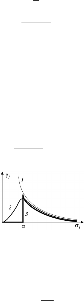
At the small singular numbers σ

in comparison with the ratio σ

/σ

(σ



/σ

), for the “usual” LSM (the ﬁrst procedure), corresponding value γ

goes up

fast, and it leads to the instability of the solution. In the cases of the statistical

regularization (the second procedure) and the singular analysis (the third procedure)

≈ 0 and γ

= 0 are valid correspondingly. At a great value of σ

(σ

 σ

/σ

)

all three methods lead to the same result.

It is necessary to point out, that the singular analysis is one of the expedients

of the regularization of the solution, and the basic diﬀerence from the estimates

obtained by the statistical regularization in a range of great values of σ

, but a little

bit larger than σ

/σ

, is the next: γ

= 0 for the singular analysis and it decreases

smoothly as

+ σ

/σ

, i = 1, . . . , S,

for the statistical regularization method (Fig. 6.1). The important result of this sec-

Fig. 6.1 Dependence of the elements of matrix Γ (6.54) on eigenvalues σ

(6.49) for an estimation

by the methods: LSM (1), statistical regularization (2), singular analysis (3).

tion consists in establishing the connection between the threshold value α, specifying

in the singular analysis using a priori data, and the noise-to-signal ratio (σ

/σ

which one is customary for an interpreter and has an explicit physical sense.

The condition measure β, introduced above, can be expressed through the min-

imum and maximum singular numbers

β =

max

min

184 STATISTICAL METHODS OF GEOPHYSICAL DATA PROCESSING

As it was mentioned, the value β can be used as a measure of the linear de-

pendence of columns of the matrix ψ

ψ. If the value of β is close to 1, then the

columns are “practically independent”. If β is suﬃciently great, then the columns

are “practically dependent”. Introducing the threshold value α reduces the con-

dition number β up to σ

max

/α, that leads to a more stable determination of the

desired parameters.

6.12.1 Resolution matrix

Let us to consider an additive model

u = ψθ +

ε. (6.55)

We introduce the matrix L, which is an “inverse” matrix with respect to the matrix

ψ and it deﬁnes a “rule” of the derivation of the estimate

θ of the vector

θ using

the vector of measured data u,

θ = Lu.

To deﬁne the resolution matrix R as a product of L and ψ

R = Lψ.

For clearing up of a sense of the resolution matrix, we multiply the left hand side

and the right hand side of the equation (6.55) by the matrix L. At tending the

values of the additive noise addend εε to zero, we obtain

θθ

ε→0

−→ Rθ.

In case of the solution of the system of the linear equations (6.55) by LSM, the

resolution matrix is an identity matrix:

L = (ψ

ψ)

−1

, R = Lψ = I.

In case of the singular decomposition (6.48) of the matrix ψ, we obtain:

R = P Σ

QΣP

= P P

= I.

6.13 The Method of Least Modulus

Together with the LSM method, for processing of the geophysical data, the method

of the least modulus is widespread. This method leads to the optimum estimates

of parameters at presence in a random noise of the outliers. With the reference to

the linear model (6.15) the method of least modulus is reduced to the minimization

of the function

λ(

θ) =

i=1

−

s=1

θ = arg min

θθ

i=1

−

s=1

|. (6.56)

Methods for parameter estimation 185

Let us note, that the method of least modulus is a special case of the maximum

likelihood method with the Laplace distribution of the random parameter vector ε.

The “tails” of the Laplace distribution fall slowly, than the “tails” of the Gaussian

distribution. At the method of least squares the weight multipliers v

have a clear

physical sense, they are in inverse proportion to the standard deviations of the

measurements.

To ﬁnd a minimum of the function λ(θ) two approaches can be used. The ﬁrst

approach is based on the linear-programming technique. The second one is the

iterative procedure based on the weighted LSM.

Let us consider the second approach in detail.

We introduce a function of two vector arguments θ

θ and ρ

(θ, ρ) =

i=1

−

s=1

−

s=1

. (6.57)

If θθ = ρ, then the function (6.57) transforms to the function (6.56):

(

θ, θ

θ) = λ(θ

θ).

The presentation (6.56) enables to create an iterative procedure for ﬁnding an esti-

mate by the method of least modulus. Let’s an initial approximation for the desired

parameter vector θ

(0)

is given. We substitute the value of θ

(0)

to the expression

(6.57) instead of the vector ρ, then

(

θ, θ

(0)

) =

i=1

−

s=1

−

s=1

(0)

, (6.58)

or, introducing the notation

−

s=1

(0)

, (6.59)

we obtain

(θθ, θ

(0)

) =

i=1

(0)

−

s=1

|. (6.60)

The quadratic form of (6.58), (6.60) explicitly corresponds to the quadratic form of

LSM. The estimate of the desired parameter vector is determined by

θ = (ψ

(0)

ψ)

−1

(0)

u, (6.61)

where W

(0)

= diag(w

, w

, . . . , w

186 STATISTICAL METHODS OF GEOPHYSICAL DATA PROCESSING

Let’s accept the estimate (6.61) as the ﬁrst approximation of the estimate for

the least modulus method:

θθ

(1)

θ,

and to use it for computing the new weight multipliers. To substitute the obtained

estimate to the expression (6.57) instead of

ρ:

(

θ, θ

(1)

) =

i=1

(1)

−

s=1

)

, (6.62)

where

(1)

−

s=1

(1)

Further, the LSM estimate we ﬁnd by minimizing of the quadratic form (6.62)

θ = (ψ

(1)

ψ)

−1

(1)

We accept this estimate as the second approximation of the estimate for the least

modulus method:

θθ

(2)

θ.

Substituting θ

(2)

to the expression (6.57) instead of θ we ﬁnd θ

(3)

. The iterative

procedure continues until at k-th step the threshold condition

|θ

(k)

− θ

(k−1)

|θ

(k)

< δ ∼ 10

−2

÷ 10

−3

is satisﬁed. Usually the value of δ is a order of 10

−2

–10

−3

The main element of the considered procedure is LSM. At each step we make

correction of the weights W

in accordance with the LSM estimate obtained at the

previous step.

6.14 Robust Methods of Estimation

Most of the considered estimation algorithms were based on the assumption of

the normal distribution of the random vector ε

ε. If this assumption is not valid,

then estimates obtained by LSM lose the optimality. Besides the LSM estimates

are sensitive to the great errors of observations. Therefore, the creation of the

algorithms, which are stable at deviations from the initial assumptions about the

model, is an actual problem. In mathematical statistics the methods of estimation,

which are stable against the deviations of the supposed distributions of the random

components from a true model are designed. These methods are called the robust

methods. Three robust algorithms will be considered below.

Methods for parameter estimation 187

6.14.1 Reparametrization algorithm

Let us consider the robust estimation algorithm for the parameter vector θθ using

the model (6.15), and based on the reparametrization of an initial model (Meshalkin

and Kurochkina, 1981). As the result of the reparametrization, the new parameters

appear as the stable ones in wide class of the noise at a deviation of their distribution

from the normal distribution. The estimation procedure looks like the next.

(1) To set an initial approach for the parameter vector θ and a variance σ

. As the

vector

an LSM estimate can be used. The variance can be estimated by the formula

(u − ψθθ

)

(u − ψ

)

n − S

(2) In k-th iteration we compute the deviation

= u

−ψψ

(k)

where ψ

is i-th row of the matrix. To determine the weight function

w(ε

) = exp



−

2ˆσ



At that we should determine a value of the constant η, which determines a width

of the weight bell-shaped function. Such value may choose by an experimental

determination. With the reference to the processing of geophysical data, this

value is advisable to put η = 0.2.

(3) To ﬁnd the estimate

θ by minimizing of the quadratic form:

λ(θθ) =

j=1

− ψ

θ)

w(e

θ = (ψ

W ψ)

−1

where W = diag(w

, w

, . . . , w

(4) To calculate the normalized weighted deviation

Y =

λ(θ)

i=1

(ε

)

(5) To ﬁnd the estimate

k+1

and dispersion ˆσ

k+1

using the equation

k+1

θθ

−1

ˆσ

(

θθ −

θθ

), (

σσ

k+1

)

−1

= Y −

ˆσ

(6) If the diﬀerence between the estimates obtained on k-th and (k+1)-th iterations

have an inessential diﬀerence, i.e.

max



k+1

−



≤ δ



ˆσ

k+1

− ˆσ

ˆσ



≤ δ

where δ

and δ

are the constants of order 10

−2

–10

−3

, then

, σ

are the

desired estimates, otherwise the iterative procedure will be repeated, starting

from the point 2. As it is shown by the numerical simulation, it needs 7–10

iterations.

188 STATISTICAL METHODS OF GEOPHYSICAL DATA PROCESSING

(7) The covariance matrix of the estimates of the desired parameters is determined

by the formula

= (ψ

W ψ)

−1

ˆσ

Described algorithm may easily be realized on a computer, because its basic

element is the weighted LSM procedure.

Let us consider two robust nonlinear estimators.

6.14.2 Huber robust method

Let’s the random components ε

in the model (6.15) are independent and equally

distributed with a symmetric density function. If the probability of a great outlier

is equal to α, then

p(n) = (1 − α)X(e) + αZ(e),

where the supposed distribution X(n) and “weed” Z(e) are the symmetric densities:

X(e) = 1 − X(−e), Z(e) = 1 − Z(−e).

Assuming that the random components have the normal distribution, we come

to a model of the crude errors, which can be applied to the static correction at

processing of seismic data. In that case instead of minimizing of a quadratic form,

for the determination of the parameter vector θθ, it is proposed to solve the next

problem (Huber, 2004):

θ = arg min

i=1

H(u

−ψ

θ), (6.63)

where H is the correspondingly chosen function.

In the general case the solution of the problem (6.63) reduces to the system of

nonlinear equations

i=1

h(u

− ψ

θθ)ψ

= 0,

where s = 1, 2, . . . , S, h(ε) = H

(ε). As the function H we can choose the next

function (Fig. 6.2)

H(ε) =



/2, |ε| < c,

c|ε| − c

/2, |ε| ≥ c.

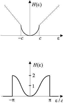
Methods for parameter estimation 189

Fig. 6.2 Huber’s proximity function between measured data and model data.

Fig. 6.3 The proximity function between measured data and model data.

6.14.3 Andrews robust method

Let us consider one more robust estimator (Andrews, 1974) where the weighted LSM

method appears as a basic element. To ﬁnd the estimate of the model parameters

by minimizing the next nonlinear function:

θ = arg min

i=1

H(u

− ψ

θ), (6.64)

where

H(ε) =



1 − cos(ε

/c), |ε

| < cπ,

0, |ε

| ≥ cπ,

(see Fig. 6.3). As the estimate ˆσ we accept a median of the absolute values:

ˆσ = med |u

− ψ

θ|.

The problem (6.64) leads to the system of linear equations

i=1

h(ε

)ψ

= 0, s = 1, . . . , S, (6.65)

h(ε

) = H

(ε

) =



sin(ε

/c)/c, |ε

| < cπ,

0, |ε

| ≥ cπ.

The solution of the system of linear equations using the iterative procedure leads

to the next steps.

190 STATISTICAL METHODS OF GEOPHYSICAL DATA PROCESSING

(1) To establish the initial vector θ

or to use for its determination LSM.

Let us consider the estimator of

k+1

, if the estimates

, k = 0, 1, . . . are

known.

(2) To calculate the deviation ˆε

= u

− ψ

(3) To ﬁnd the estimate ˆσ

= med ˆε

(4) To calculate the weight function



[sin(ˆε

/c)/c][ˆε

]

−1

, |ε

|/c < π,

0, |ε

|/c ≥ π.

(5) To solve the system of equations (6.65), which can be represented in the form

i=1

= 0.

i=1

− ψ

(k+1)

) = 0.

Using the weighted LSM to obtain the estimate

k+1

= (ψ

ψ)

−1

where W = diag(w

, w

, . . . w

(6) To check an accuracy of the obtained estimates

max

sk+1

−

≤ δ

|ˆσ

k+1

− ˆσ

|ˆσ

≤ δ

where δ

and δ

are the values of the order 10

−2

–10

−3

. If the inequalities are

satisﬁed, then θ

and ˆσ

are the desired estimates. If not, we continue the

procedure from the point 2. For the case of the real data the recommended

value of c is 1,5.

The essential diﬀerence of this method from the reparametrization algorithm is

that for a great deviation the value of the weight function puts to zero.

6.15 Interval Estimation

We have considered some examples of the point estimation. In practice the interval

estimation, which is intimately connected with the point estimation, is widespread

as well. The interval estimation gives not only a numerical value of parameters,

but also it produces an accuracy and reliability of the estimation. So, for example,

at treating experimental data the great interest is introduced by a problem of the

deﬁnition of an interval, in which one the true value of parameter lays with the

given probability. The problems of a such type are solved by the interval estimation

method.

Methods for parameter estimation 191

Let’s the estimate

θ is unbiased estimate of the parameter θ. To establish enough

great probability β (β = 0.9, . . . , 0.95), we ﬁnd an admissible deviation value δ of

and θ:

P (|

θ − θ| < δ) = β, (6.66)

Moreover, the deviations exceeding on an absolute value of δ, occur with the small

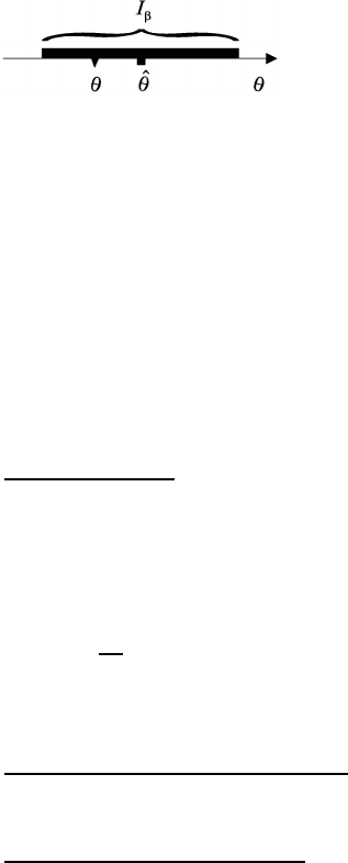
probability 1 −β. The expression (6.66) can be represented as

P (

θ − δ < θ <

θ + δ) = β. (6.67)

This inequality yields that with the probability β the random interval I

= [

θ −

δ,

θ + δ] covers a true value of the parameter (Fig. 6.4). The probability β is usually

Fig. 6.4 The conﬁdence interval I

and estimated parameter

θ.

called the conﬁdence probability,, and the random interval [

θ − δ,

θ + δ] is called

the conﬁdence interval. As it follows from the expression (6.67), to determine the

conﬁdence interval it is necessary to know a probability distribution of the estimate.

As it was already mentioned, in the case of the normal distribution an error vector

of the estimates obtained by LSM in case of the linear model (6.15) have the normal

distribution, i.e.

i = θ

, R

= σ

[(ψ

W ψ)

−1

]

s = 1, 2, . . . , S.

Each component of the estimating parameter vector

has the normal distribution

with the mathematical expectation θ

and the variance σ

[(ψ

ψ)

−1

]

− θ

[(ψ

W ψ)

−1

]

1/2

∈ N (0, 1). (6.68)

To introduce the deviation vector

ˆε

ε =

u−ψ

θ and the quadratic form of deviation

εε

ˆε

ε. The random vector

θ is S-dimensional normal vector, and the random vector

εε is (n−S)-dimensional normal vector. These vectors are independent. The random

value

ˆε

ε (6.69)

has the distribution χ

n−S

and does not dependent on

θ.

Using the relations (6.68) and (6.69), to build the variable

n−s

− θ

[(ψ

W ψ)

−1

]

1/2

εε

εε/(n − S)

1/2

− θ

(ψ

W ψ)

−1

ε/(n − S)

1/2

192 STATISTICAL METHODS OF GEOPHYSICAL DATA PROCESSING

which is a ratio of a random variable with the normal distribution (N(0, 1)) and a

sum of squared normally distributed variables with a number of degrees of freedom

n − S. Such variable has the Student’s distribution with a number of degrees of

freedom n − S and it enables to create the conﬁdence interval for θ

To specify the conﬁdence probability β. For given dimensions of the observed

data vector and the desired parameter vector S to determine a number of degrees of

freedom k = n − S. The values of k and β are an input data for the determination

of γ, such that

P [|t

n−S

| ≤ γ] = β.

The conﬁdence interval with the conﬁdence probability β describes by the formula

± γ[(ψ

W ψ)

−1

]

1/2



εε

n − S



1/2

or, taking into account, that

ˆσ

n − S

, ˆσ

= ˆσ

[(ψ

W ψ)

−1

]

we obtain

= [

± γˆσ

]. (6.70)

From an analysis of the formula (6.70) follows that the conﬁdence interval de-

termines both the conﬁdence probability and an accuracy of the estimate. Together

with the interval estimations of the parameters, a practical importance possesses es-

timation of the conﬁdence bounds for an approximated function. Let’s deterministic

component of a model with a true parameter vector is written as

ff = ψθθ, (6.71)

where the estimate of the function f, obtained by the substitution to the right hand

side of equality (6.71) the LSM estimate of the vector

θ, can be written as

ff = ψ

θθ.

Let’s note, that

ff does not depend on

ε. To deﬁne the function t

n−S

as a

ratio of the variable

− f

[ψ(ψ

W ψ)

−1

]

1/2

with the normal distribution and the variable

ˆε

n − S

ˆσ

The square of this variable belongs to χ

n−S

distribution with n − S degrees of

freedom:

n−S

− f

[ψ(ψ

W ψ)

−1

]

1/2

[

ˆε

ε/(n − S)]

1/2

∈ St (t