Wai-Fah Chen.The Civil Engineering Handbook
Подождите немного. Документ загружается.


Urban Transit
61
-3
Other Modes
Trolleybus coaches resemble diesel coaches, except that they are powered by electric motors, drawing
electric current from overhead wires. They are common in Europe and operate in several North American
cities. Their virtually unlimited power enables them to accelerate more quickly and climb steep hills more
easily than diesel buses, and because they need no transmission, their ride is smoother. Fumes are
eliminated, improving the environment and making it easier for them to operate in tunnels. The overhead
wires, however, are sometimes seen as a detriment to the environment. Trolleybuses are not as flexible
as diesel buses — they must be replaced by diesel buses when there is a detour, for example — but they
can maneuver around a blocked lane, making them better suited to mixed traffic than light rail. The cost
of the power line network generally limits them to high-volume routes, since the benefits of electrification
are proportional to the number of passengers and vehicles on the route.
A more recent bus variation is the self-steering bus, guided by contact between a raised curb and small
guide wheel that extends from the side of the bus. It allows a bus to operate in a smaller lane, lowering
construction costs on elevated busways and in tunnels.
Commuter rail has long been used in older U.S. cities for long-distance commuting. Extensions are being
built, and new systems have recently been opened in metropolitan Washington, in Los Angeles, and in south
Florida. They use standard locomotives (electric or diesel) pulling passenger cars on rail lines often shared
with freight or long-distance passenger traffic. More than any other mode, commuter rail relies on auto
access at the suburban end of the trip and usually relies on metro for distribution at the downtown end.
The design and operation of downtown terminals where many lines converge can be quite involved.
Numerous other transit modes operate in different cities. They include ferry boat, cable car, incline,
and, more recently, downtown people mover.
Line Capacity
The line capacity of a transit line is the number of passengers that can be carried per hour in one direction
past any point. Line capacity is often a major consideration of choice of mode for a new transit line. If
there is no shortage of vehicles, the line capacity is constrained only by the headway (time interval)
between vehicles:
(61.1)
Vehicle capacity includes standees, according to the level of crowding deemed acceptable. Minimum
headway is a function of safety and is governed primarily by vehicle interference at stations. For example,
a metro with 6-car trains that can fit 240 people per car, if operating at a 4-min headway, can carry
21,600 pass/h in each direction; at a 2-min headway, line capacity is doubled. Typical line capacities for
various modes are given in Table 61.2. By contrast, a freeway lane with headways of about 1.8 s and
average occupancy of 1.2 persons carries only 2400 people per hour. If that lane were converted to a
TA BLE 61.2
Typical Line Capacities
Tr ain Minimum Line
Mode Size Headway Occupancy Capacity
Auto on freeway 1 1.8 s 1.2 2,400/h/lane
High-occupancy freeway lane (5% buses) 1 2 s 5 9,000/h
Bus-only freeway lane 1 4 s 40 36,000/h
Bus in arterial bus lane 1 30 s 65 7,800/h
Busway 1 20 s 60 10,800/h
Light-rail exclusive way 2 1 min 150 18,000/h
Metro62 min 240 43,200/h
Commuter rail 10 10 min 275 13,750/h
Line capacity Vehicle capacity Train size Minimum headway
pass h pass veh
veh s
() ( )
() ()
=¥¥3600
© 2003 by CRC Press LLC

61
-4
The Civil Engineering Handbook, Second Edition
high-occupancy vehicle lane, with an average occupancy of 5 (95% carpools, 5% buses), then even with
half the vehicular volume its passenger volume would more than double and its line capacity would
almost quadruple, since the minimum headway would only barely increase.
Comparing Alternatives
Many studies have been done comparing transit alternatives. There is no clear consensus on the superi-
ority or inferiority of any mode in a general sense. Any investment using federal funds requires an
alternative analysis
that considers a no-build alternative (including low-cost transportation systems
management improvements) and at least two different modes, with variations in alignment for each.
Basic analysis is done using methods described in Chapter 58. Evaluation of alternatives is done following
federal guidelines considering capital cost, operating cost, expected number of new passengers, benefits
to existing passengers, and financing and political considerations [Zimmerman, 1989]. As a rule of thumb,
construction cost for elevated exclusive guideway is 2 to 3 times greater than for at-grade, and subway
is 4 to 10 times more costly than at-grade, creating a strong incentive to utilize existing rail rights-of-
way and other alignments that avoid the need for tunneling or aerial construction.
61.2 The Transit Environment
Travel Patterns and Urban Form
Between about 1870 and 1940, streetcar (first horse drawn, later electric) was the primary mode of urban
travel. Consequently, urban development during this period was oriented around streetcar use — dense
development along radial streetcar lines, with a heavy concentration of commercial development in the
central business district (CBD). Postwar development, in contrast, has been largely auto-oriented. At first
homes, later stores, and finally employers became dispersed in large numbers in the suburbs. The travel
patterns of streetcar-era development — many to one or many to many along a linear corridor — lend
themselves to the kind of demand concentration that transit can serve easily. The dispersed travel patterns
of auto-oriented urban land use are far more difficult for transit to serve [Pushkarev and Zupan, 1977].
A transit system in an older city with a concentrated urban form faces far different problems than one
serving a dispersed urban form. The former can face challenges such as how to carry the enormous
demand; the main challenge in the latter is how to attract passengers.
Historically, as trip ends dispersed and income and auto ownership increased, transit ridership
declined. “Captive” markets, primarily the carless poor and persons unable to drive, have shrunk. Within
the “choice” market, discretionary trips (e.g., shopping trips that can be arranged to be done when an
auto is available and where parking is free) were hardest hit. In cities with large downtown employment,
parking is expensive, and the home-to-work commute market has held its own and in some cases grown.
As a result, transit demand in large cities has become more and more peaked. The
peak-to-base ratio
(the
number of buses in service during the a.m. peak period divided by the number in service during the
base period) can be as great as 3:1. Passenger utilization is still more peaked because vehicles are more
crowded during peak hours. This level of peaking hurts transit’s economy because fixed facilities are
underutilized and because of the costs inherent in starting and stopping service.
Transit Financing
Although transit first developed as a profitable private enterprise, inflation coupled with politically
mandated caps on fares and competition from autos began to cripple the industry by the end of the first
World War, leading to consolidation, disinvestment (e.g., abandoning streetcar lines, not replacing aging
vehicles), public subsidy, and eventually public ownership. The chief reasons for transit’s not being
profitable are:
© 2003 by CRC Press LLC

Urban Transit
61
-5
•
Low fare.
Political pressure has kept fares low for a variety of reasons, including accommodating
poor riders and providing an alternative to autos which, transit proponents argue, are heavily
subsidized.
•
Low demand and highly peaked demand.
These factors prevent transit from achieving economies
of scale.
•
Social service.
It is politically mandated that service be offered on routes and at times of low
demand.
•
High wages.
All large transit systems are unionized. When a large percentage of downtown workers
use transit, the threat of a strike gives unions considerable bargaining power, which they have used
effectively to negotiate high wages.
•
Restrictive work rules and various management problems.
These factors have also been blamed for
transit’s financial losses.
Capital costs are financed entirely by government subsidy. In the U.S. the Federal Transit Administra-
tion (FTA) usually covers 80%, with state and local government covering the remainder. For major
construction projects, limited federal funds sometimes result in a smaller federal share. Public subsidies
cover, as a national average, about 50% of operating costs in the U.S., although they vary a great deal
from city to city. The federal contribution is small except in small cities; state and local governments
cover most of the operating deficit. Instability in the source of state and local funding is a cause of much
uncertainty in management in many cities.
Transit Management
Ownership of public transit agencies is exercised through a board of directors whose members usually
represent the local political constituencies (cities, counties, etc.) that subsidize it. Because the board
members are political appointees, many have little knowledge about managing a transit system. Because
these members carry with them political views that sometimes conflict with one another, management
can be politically charged, making the direction unstable. For example, urban board members may want
to keep fares low, whereas suburban board members may be primarily concerned with reducing subsidies.
Construction projects always entail significant political interest. Depending on how the balance of power
changes, direction may change often.
The chief executive officer, usually called the
general manager,
is appointed by the board. The organi-
zation is usually divided functionally into departments such as transportation, maintenance, finance,
administration, planning, real estate, and construction. Larger agencies may use a modal breakdown
(bus, rail, etc.), as well, which may be under or above the functional division.
61.3 Fundamentals of Cyclic Operations
Most transit services are cyclical: vehicles leave a depot, cycle over a given route, return, and then make
another cycle. Routes that go back and forth between two terminals can still be considered cyclic, and
either terminal can be considered the depot. This section looks at a route during a period of the day in
which ridership and running times can be treated as constant.
Fundamental Operating Parameters and Relationships
Cycle time (
c
) is the time a vehicle uses to perform the cycle and wait for the next cycle. It consists of
running time and layover (or recovery) time. On routes with two terminals, layover time is usually
distributed between the two terminals. Its primary purpose is to serve as a buffer for run-time delays,
reducing the degree to which delays propagate from one cycle to the next. It also allows vehicle operators
a rest. On short urban bus routes, layover is commonly 15 to 20% of running time; on longer routes or
© 2003 by CRC Press LLC

61
-6
The Civil Engineering Handbook, Second Edition
routes with less traffic congestion, 10% is typical. Layover may be further increased by schedule slack,
as discussed later.
The service frequency (
q
) is the number of cycles per hour, the number of trips per hour passing a
given point in a given direction. (
Trip
in transit terminology refers to vehicle trips, unless otherwise
designated.) The reciprocal of frequency is headway (
h
), the time between successive trips.
If a route is operated in isolation, one can speak of the number of vehicles (
n
) operating on the route.
In the rail context,
n
is the number of trains. The fundamental relationship is
(61.2a)
(61.2b)
(61.2c)
For example, to operate a route with a 4-min cycle at a 10-min headway (a frequency of 6/h) will require
4 vehicles. Or, given 6 vehicles and a 4-min cycle, the route can operate with a 6.67-min headway (a
frequency of 9/h).
Fundamental Measures of Passenger Demand
An origin–destination (O–D) matrix — showing the number of passengers per hour traveling from one
stop to another — is the fundamental descriptor of passenger demand on a route. (Further detail, such
as fare category, usually does not matter for operations planning.) On routes operating between two
terminals, it is best to divide the demand by direction, resulting in a triangular O–D matrix for each
direction. The row and column totals represent the ons and offs (boardings and alightings) at each stop.
The grand total is the boardings (
b
) on the route.
The volume profile is the passenger volume on each interstop segment on the route. On routes that
empty out at a terminal, the volume profile is easily constructed stop by stop, beginning at the terminal,
accumulating ons and deducting offs. On loop routes that do not empty out (e.g., a circumferential route),
the volume on a segment is the sum of the demands in the O–D cells that involve travel over that segment.
Once the volume on any one segment is calculated, the volume on the succeeding segments can be found
by accumulating ons and deducting offs. The peak volume segment (also called
peak load point
or
peak
point
) is the segment with the greatest volume; its volume is the peak volume (
v
*
). On bidirectional routes,
the direction with the greater peak volume is the peak direction, and its peak volume is the route’s peak
volume. Another measure of demand is passenger-miles (or passenger-km), most easily calculated by
multiplying the volume on each segment by the segment length and summing over all segments:
(61.3)
The main quantifiable measures of service quality for transit passengers are travel time (in vehicle);
waiting time, which is approximately half the headway when service is regular and headway is not too
large; number of transfers; and level of crowding.
Basic Schedule Design
The simplest practical scheduling method involves three constraints in addition to the fundamental
relationship [Eq. (61.2)]. First, the average vehicle load at the peak point, called
peak load
(
l
p
), must not
exceed a design capacity (
k
), which depends on the size of the bus as well as standards of comfort and safety:
(61.4)
cnhnq==
nchcq==
hqcn==1
pass-mi (or pass-km) Volume on segment Length of segment =
()()
Â
ii
l
v
q
k
p
=£
*
© 2003 by CRC Press LLC

Urban Transit
61
-7
Second, the headway is usually restricted to a set of acceptable values, {
h
}. This set is based on four
considerations: (1) whole minute headways are usually required because schedules are written in whole
minutes (exception: some rail systems use the half-minute or quarter-minute as the basic unit);
(2) multiples of 5 min are desired for long headways; (3) headways that repeat every hour (e.g., 12, 15,
20, 30 min) are desirable; and (4) there is a maximum headway, called a
policy headway,
that may not
be exceeded, usually 60 min but sometimes 30 min or smaller in peak periods. For example, one set of
acceptable headways might be
(61.5)
while a more restrictive set might be
(61.6)
Third, the number of vehicles must be an integer (unless the route is not operated in isolation, in which
case scheduling must be done jointly for a number of routes, as discussed in Section 61.5). The result of
these last two constraints is to force additional slack into the schedule, in the form of both excess capacity
and excess layover.
Schedule design usually begins with a given peak volume and a given minimum cycle time (
c
min
) that
accounts for running time and minimum necessary layover. The schedule design procedure that follows
has as its primary objective minimizing fleet size (about the same as minimizing cost); its secondary
objective, for a given fleet size, is to maximize service frequency (maximize service quality). In what
follows, [ ]
+
means round up and [ ]
–
means round down. This procedure assumes that cycle times and
headways are in minutes, while frequencies and passenger volumes are hourly.
Step 1.
h
max
= [
k
/(
v
*
/60)]
–
(round down to next acceptable headway)
Step 2.
n
= [
c
min
/
h
max
]
+
Step 3.
h
= [
c
min
/
n
]
+
(round up to next acceptable headway)
Step 4.
Given
n
and
h
, determine the remaining parameters (
c, q, l
p
) using Eqs. (61.2) and (61.4). The
difference between
c and c
min
, called schedule slack, is added to the layover.
The rounding involved in steps 1 and 2 can add substantially to operating cost. For example, consider
a route for which v* = 260/h, c
min
= 51 min, and k = 50. If one ignores rounding, the minimal service
frequency is 260/50 = 5.2/h, the headway is 60/5.2 = 11.5 min, and the number of vehicles needed is
51/11.5 = 4.4. While this kind of analysis can be done in sketch planning, it does not produce a workable
design. Following are two designs using the preceding procedure; their difference is that one uses set {h
I
},
which allows an 11-min headway, while the other uses {h
II
}, which does not.
This example demonstrates the substantial effect of rounding. In case I, rounding increased fleet
requirements from the sketch planning value of 4.4 to 5. The extra resources consumed are manifest as
slack in the cycle time (the final cycle time, 55 min, is 4 min greater than required) and in slack capacity
(peak load, 47.7, is below the allowed capacity of 50). Case II, by not permitting an 11-min headway,
requires more rounding, increasing the vehicle requirement to 6. However, the extra resources are not
all wasted but are partially converted into extra service as service frequency increases, reducing passenger
Set of h
max
Acceptable Unrounded h
max
nhc
Case Headways (min) (min) Unrounded n (min) (min) l
p
I{h
1
} 11.5 11 4.64 5 11 55 47.7
II {h
II
} 11.5 10 5.1 6 9 54 39.0
h
I
{}
=º
{}
12 2025 30 35 40 45 50 55 60,, , ,,,,,,,,
h
II
{}
=º
{}
12 1012 15 20 30 60,, , ,,,,,
© 2003 by CRC Press LLC
61-8 The Civil Engineering Handbook, Second Edition
waiting time and crowding. Case II also illustrates the role of step 3 in achieving the secondary objective
of maximizing service level. Step 3 could have been omitted, leaving h = h
max
= 10 min, and the result
would have been a viable design. However, the rounding involved in calculating n (step 2) made a better
value of h (9 min vs. 10 min) possible without adding a vehicle.
Finally, a schedule with a large amount of slack time in the cycle begs for opportunities to adjust the
minimum cycle time, either lowering it enough to save a vehicle (e.g., by eliminating a deviation or
securing traffic improvements) or lengthening it by an amount less than or equal to the slack in an effort
to attract new passengers (e.g., extending the route or adding a deviation) without increasing the fleet
requirement.
Example 61.1
A downtown circulator on its own right-of-way with six tops is being planned. Stops, numbered clockwise,
are 0.5 mi apart, and travel time (including dwell time at stops) is 1.5 min per segment, for a 9-min
overall running time. There should be little or no layover because of the nature of the service; likewise,
the only restriction on headway is that it be in quarter minutes. Vehicle design capacity is 40. Two
alternative configurations are to be compared. Alternative A is service in the clockwise direction only.
Alternative B is service in both directions; naturally, alternative B involves a greater construction cost.
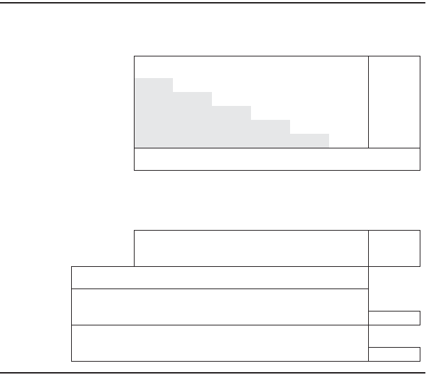
Estimated p.m. peak demand is shown in the O–D matrix in Table 61.3(a). For alternative A the volume
on segment 6-1 is the sum of the cells in the O–D matrix that involve travel over that segment; those
cells are shaded in Table 61.3(a). Volume on the remaining segments is found by accumulating ons and
subtracting offs, resulting in the volume profile shown in Table 61.3(b). Peak volume is seen to be 1333/h.
Multiplying volume by segment length and by segment travel time results in passenger-miles and pas-
senger-minute estimates.
TA BLE 61.3 Demand Analysis, One-Directional Circumferential Route
a. Origin–Destination Matrix (passengers/hr)
\ TO 123456TOTAL
FROM \
1 150 150 300 150 150 900
2 100 50 100 50 50 350
3 100 33 100 50 50 333
4
200 67 67 67 67 467
5 100 33 33 33 50 250
6 100 33 33 33 33 233
TOTAL 600 317 333 567 350 367 2533
b. Vo lume Profile
SEGMENT
AFTER STOP 6 123456TOTAL
OFF 600 317 333 567 3501 367 2533
ON 900 350 333 467 250 233 2533
VOLUME 1000 1300 1333 1333 1233 1133 1000
MILES 0.5 0.5 0.5 0.5 0.5 0.5
PASS-MI 650 667 667 617 567 500 3667
MIN 1.5 1.5 1.5 1.5 1.5 1.5
PASS-MIN 1950 2000 2000 1850 1700 1500 11000
Note: Vo lume on first segment shown is sum of shaded cells in O–D matrix.
© 2003 by CRC Press LLC
Urban Transit 61-9
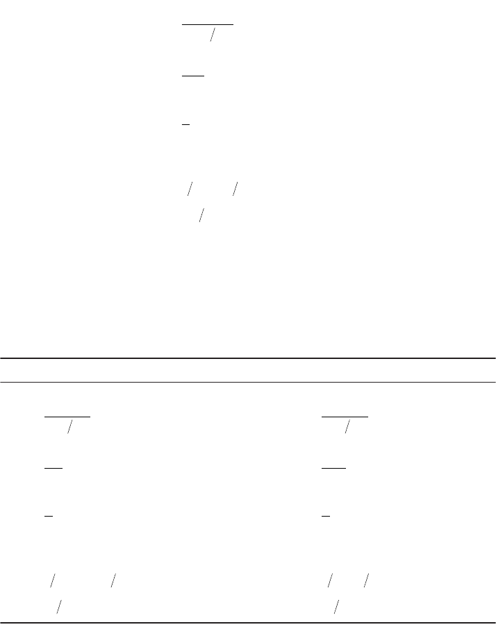
Following the four steps for schedule design,
For alternative B demand must be split between the two directions. Assuming that passengers choose the
shortest direction and that those traveling three stops split themselves evenly between the two directions,
O–D matrices for the two routes are shown in Table 61.4(a). Volume profiles [Table 61.4(b)] are con-
structed as they were for alternative A, with the shaded cells in the corresponding O–D matrix constituting
load on the first segment. The peak volumes are 517/h on the clockwise route and 550/h on the coun-
terclockwise route. Schedule design for the two routes is as follows:
A comparison between alternatives A and B is given in Table 61.5. Most of the table is self-explanatory.
Averages in rows 3, 5, 8, and 10 are found by dividing the previous figure by total boardings (row 1).
Average wait time in row 6 is taken to be half the headway; total wait (row 7) is the product of the average
and the total boardings. In some alternative analyses, wait time is weighted more heavily than travel time;
this measure has not been taken in this example. In comparing the two examples, one can see that
alternative B requires one fewer vehicle and involves less passenger time overall. A decision between the
two alternatives should consider other factors as well, including vehicle requirements in other periods,
capital costs, operating statistics in other periods and in the future, and sensitivity to changes in the
demand estates.
Clockwise route Counterclockwise route
h
n
h
c
q
l
p
max
..min
.
.
..min
. min,
.
.
=
()
È
Î
Í
Í
˘
˚
˙
˙
=
[]
=
=
È
Î
Í
˘
˚
˙
=
[]
=
=
È
Î
Í
˘
˚
˙
=
[]
=
=
()()
==
==
==
-
-
+
+
+
+
40
1333 60
180 175
9
175
514 6
9
6
15 15
15 6 9 0
60 1 5 40
1333 40 33 3
and layover
h
h
n
h
c
q
l
p
max
..min
.
. min
. min,
..
..
=
()
È
Î
Í
Í
˘
˚
˙
˙
=
[]
=
=
È
Î
Í
˘
˚
˙
=
=
È
Î
Í
˘
˚
˙
=
=
()( )
==
==
==
-
-
+
+
40
517 60
464 45
9
45
2
9
2
45
245 9 0
60 4 5 13 33
517 13 33 38 8
layover
h
h
n
h
c
q
l
p
max
..min
.
.
min
min,
.
=
()
È
Î
Í
Í
˘
˚
˙
˙
=
[]
=
=
È
Î
Í
˘
˚
˙
=
[]
=
=
È
Î
Í
˘
˚
˙
=
=
()()
==
==
==
-
-
+
+
+
40
550 60
436 425
9
425
212 3
9
3
3
33 9 0
60 3 20
550 20 27 5
layover
h
© 2003 by CRC Press LLC
61-10 The Civil Engineering Handbook, Second Edition
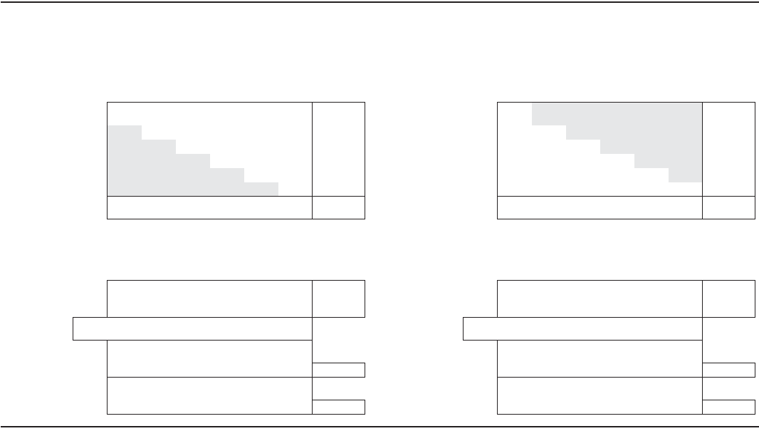
TA BLE 61.4 Demand Analysis, Two Circumferential Routes
CLOCKWISE ROUTE COUNTERCLOCKWISE ROUTE
a. Origin–Destination Matrix (passengers / hr)
\ TO 123456TOTAL \ TO123456TOTAL
FROM / FROM \
1 150 150 150 0 0 450 1 0 0 150 150 150 450
2 050100 25 0 175 2 100 0 0 25 50 175
3 0 0 100 50 25 176 3 100 33 3 3 25 158
4 100 0 06767233 4 100 67 67 0 0 233
5 100 17 0 050167 5 0 17 33 33 083
6
100 33 17 0 0 150 6 0 0 17 33 33 83
TOTAL 300 200 217 350 142 142 1350 TOTAL 300 117 117 217 208 225 1183
b. Vo lume Profile
SEGMENT SEGMENT
AFTER STOP 6 123456 TOTAL AFTER STOP 1654321TOTAL
OFF 300 200 217 350 142 142 1350 OFF 225 208 217 117 117 300 1183
ON 450 175 175 233 167 150 1350 ON 83 83 233 158 175 450 1183
VOLUME 367 517 492 450 333 358 367 VOLUME 550 408 283 300 342 400 550
MILES 0.5 0.5 0.5 0.5 0.5 0.5 MILES 0.5 0.5 0.5 0.5 0.5 0.5
PASS-MI 258 246 225 167 179 183 1258 PASS-MI 204 142 150 171 200 275 1142
MIN 1.5 1.5 1.5 1.5 1.5 1.5 MIN 1.5 1.5 1.5 1.5 1.5 1.5
PASS-MIN 775 737 675 500 538 550 3775 PASS-MIN 612 425 450 512 600 825 3425
Note: volume on first segment is sum of shaded cells in O–D matrix.
© 2003 by CRC Press LLC
Urban Transit 61-11
61.4 Frequency Determination
Most bus, light rail, and metro routes operate at a constant headway over a time period. When demand
is very low, routes follow a policy headway (H), the maximum headway allowed by system policy. When
demand is very high, the headway is set so that average peak load equals or is just below the design
capacity, as described in Section 61.3.
In between very low and very high demand, there is no widely accepted method for setting frequencies.
An optimization framework, based on a tradeoff between operator cost and passenger waiting time,
provides a rule that can be used to consistently set frequencies on routes. Let
Assuming that wait time is half the headway, the combined operator plus passenger cost per hour for
route i is
Summing over all routes and then minimizing by setting to zero the derivative with respect to q
i
yields
the “square root rule”:
(61.7)
Incorporating policy headway and capacity constraints, the rule has two modifications:
•If the solution is below 60/H, set q
i
= 60/H (use policy headway).
•If the solution is below v
*
i
/k, set q
i
= v
*
i
/k (make peak load equal capacity).
In addition, solutions must be rounded appropriately to satisfy integer constraints as described earlier.
The value of time can be explicitly specified as a matter of policy (one half the average wage is typical).
Alternatively, it can be implicitly determined by a constraint on total operating cost per hour of system
operation [(OC) Â c
i
q
i
£ Budget], in which case the value of time will be that value for which the total
operating cost when the q
i
values are set by the constrained square root rule equals the budget [Furth
and Wilson, 1981]. The framework can be further generalized by recognizing that demand is not fixed
TA BLE 61.5 Comparison of Alternatives
Alternative A
Alternative B
Clockwise Counterclockwise Total
1. Boardings (pass/h) 2,533 1350 1183 2,533
2. Passenger-miles (per/h) 3,667 1258 1142 2,400
3. Average trip length (mi) 1.45 0.95
4. Travel time (pass-min/h) 11,000 3775 3425 7,200
5. Average ride time (min) 4.34 2.84
6. Average wait time (min) 0.75 2.25 1.5
7. Total wait time (pass-min/h) 1,900 3038 1775 4,812
8. Average wait time (min) 0.75 1.90
9. Total pass-min per h 12,900 12,012
10. Average travel + ride time (min) 5.09 4.74
11. Vehicles needed 6 2 3 5
OC operating cost per vehicle hour $ veh-h
VOT value of passenger wait time $ pass-h
()
=
()
()
=
()
OC VOT
()
+
()
cq b q
ii i i
05.
q
b
c
i
i
i
=
()
()
05. VOT
OC
© 2003 by CRC Press LLC
61-12 The Civil Engineering Handbook, Second Edition
but will respond to frequency changes, so the generalized cost function should include the societal benefit
of increased ridership and consumer surplus. However, nearly the same result will be reached if demand
is treated as constant because the goals of minimizing waiting time for existing passengers and trying to
attract new passengers are so much in harmony. If the driving limitation is number of vehicles of varying
types instead of an operating cost budget, the same framework applies, with OC = 1 and Budget equal
to fleet size. A useful dynamic programming solution to the latter problem using a similar optimization
framework is found in Hasselstrom [1981]; unlike the calculus-based models, it yields solutions that do
not need to be rounded.
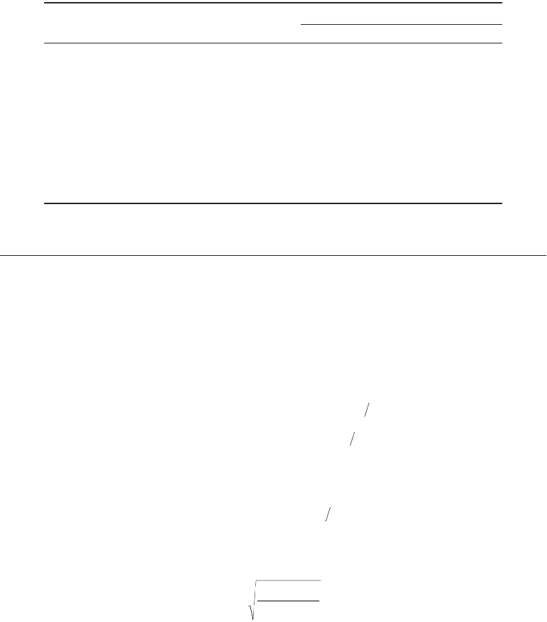
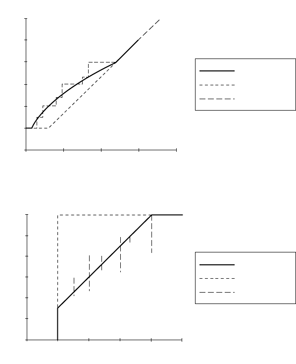
Figure 61.1 depicts graphically how the constrained square root rule applies to routes with varying
levels of ridership in comparison with minimum cost scheduling, using typical values for OC ($60/veh-h),
c
i
(1h), H (60 min), k (60), VOT ($4/hour), and the ratio v
*
i
/b
i
(0.5). Part (a) shows how frequency varies
with ridership; part (b) shows how peak load varies with frequency.
The cures have three ranges:
1. For low-volume routes, policy headway governs; frequency is independent of passenger volume;
increases in ridership are simply absorbed by increasing load.
2. For intermediate-volume routes, the square root formula applies; frequency increases with pas-
senger volume, though less than proportionally, because part of the passenger volume increase is
FIGURE 61.1 Frequency determination rules.
6
5
4
3
2
1
0
0 100 200 300 400
Frequency
(a) Frequency vs. peak volume
Peak volume
(b) Peak load vs. frequency
60
50
40
30
20
10
0
012345
Peak load
Frequency
Square root
Minimum cost
Graduated
Square root
Minimum cost
Graduated
© 2003 by CRC Press LLC