Wai-Fah Chen.The Civil Engineering Handbook

Подождите немного. Документ загружается.

18-10 The Civil Engineering Handbook, Second Edition

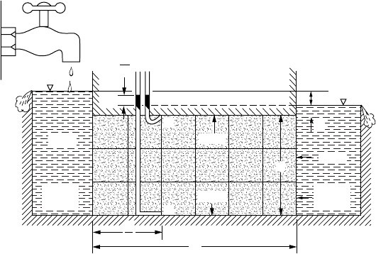
of discharge through the section Q and the head loss (h = 16 ft) must be constant. If the ﬂow region

is saturated, it follows that the two impervious boundaries are streamlines and their difference must be

identically equal to the discharge quantity

From among the inﬁnite number of possible streamlines between the impervious boundaries, we

sketch only a few, specifying the same quantity of ﬂow between neighboring streamlines. Designating N

as the number of ﬂow channels, we have, from above,

Similarly, from among the inﬁnite number of possible equipotential lines between headwater and

tailwater boundaries, we sketch only a few and specify the same drop in head, say, Dh, between adjacent

equipotential lines. If there are N

equipotential drops along each of the channels,

(18.24)

If, now, we also require that the ratio Dw/Ds be the same at all points in the ﬂow region, for convenience,

and because a square is most sensitive to visual inspection, we take this ratio to be unity,

and obtain

(18.25)

Recalling that Q, k, and h are all constants, Eq. (18.25) demonstrates that the resulting construction,

with the obvious requirement that everywhere in the ﬂow domain streamlines and equipotential lines

meet at right angles, will yield a unique value for the ratio of the number of ﬂow channels to the number

of equipotential drops, N

. In Fig. 18.8 we see that N

equals about 5 and N

equals 16; hence, N

5/16.

The graphical technique of constructing ﬂow nets by sketching was ﬁrst suggested by Prasil [1913]

although it was developed formally by Forchheimer [1930]; however, the adoption of the method by

engineers followed Casagrande’s classic paper in 1940. In this paper and in the highly recommended ﬂow

nets of Cedergren [1967] are to be found some of the highest examples of the art of drawing ﬂow nets.

Harr [1962] also warrants a peek!

Unfortunately, there is no “royal road” to drawing a good ﬂow net. The speed with which a successful

ﬂow net can be drawn is highly contingent on the experience and judgment of the individual. In this

regard, the beginner will do well to study the characteristics of well-drawn ﬂow nets: labor omnia vincit.

In summary, a ﬂow net is a sketch of distinct and special streamlines and equipotential lines that preserve

right-angle intersections, satisfy the boundary conditions, and form curvilinear squares.

The following

procedure is recommended:

There is little to be gained by retaining the approximately equal sign ª.

We accept singular squares such as the ﬁve-sided square at point H in Fig. 18.8 and the three-sided square at

point G. (It can be shown — Harr [1962], p. 84 — that a ﬁve-sided square designates a point of turbulence). With

continued subdividing into smaller squares, the deviations, in the limit, act only at singular points.

BGHC

–=

QD kN

-------

hD==

h and QD k

------

-------

h==

------- 1=

------

Groundwater and Seepage 18-11

1. Draw the boundaries of the ﬂow region to a scale so that all sketched equipotential lines and

streamlines terminate on the ﬁgure.

2. Sketch lightly three or four streamlines, keeping in mind that they are only a few of the inﬁnite

number of possible curves that must provide a smooth transition between the boundary streamlines.

3. Sketch the equipotential lines, bearing in mind that they must intersect all streamlines, including

boundary streamlines, at right angles and that the enclosed ﬁgures must form curvilinear rectan-

gles (except at singular points) with the same ratio of Ds/Ds along a ﬂow channel. Except for partial

ﬂow channels and partial head drops, these will form curvilinear squares with Dw = Ds.

4. Adjust the initial streamlines and equipotential lines to meet the required conditions. Remember

that the drawing of a good ﬂow net is a trial-and-error process, with the amount of correction

being dependent upon the position selected for the initial streamlines.

Example 18.1

Obtain the quantity of discharge, Q/kh, for the section shown in Fig. 18.9.

Solution. This represents a region of horizontal ﬂow with parallel horizontal streamlines between the

impervious boundaries and vertical equipotential lines between reservoir boundaries. Hence the ﬂow net

will consist of perfect squares, and the ratio of the number of ﬂow channels to the number of drops will

be N

= a/L and Q/kh = a/L.

Example 18.2

Find the pressure in the water at points A and B in Fig. 18.9.

Solution. For the scheme shown in Fig. 18.9, the total head loss is linear with distance in the direction

of ﬂow. Equipotential lines are seen to be vertical. The total heads at points A and B are both equal to

2h/3 (datum at the tailwater surface). This means that a piezometer placed at these points would show

a column of water rising to an elevation of 2h/3 above the tailwater elevation. Hence, the pressure at

each point is simply the weight of water in the columns above the points in question: p

= (2h/3 + h

+ a)g

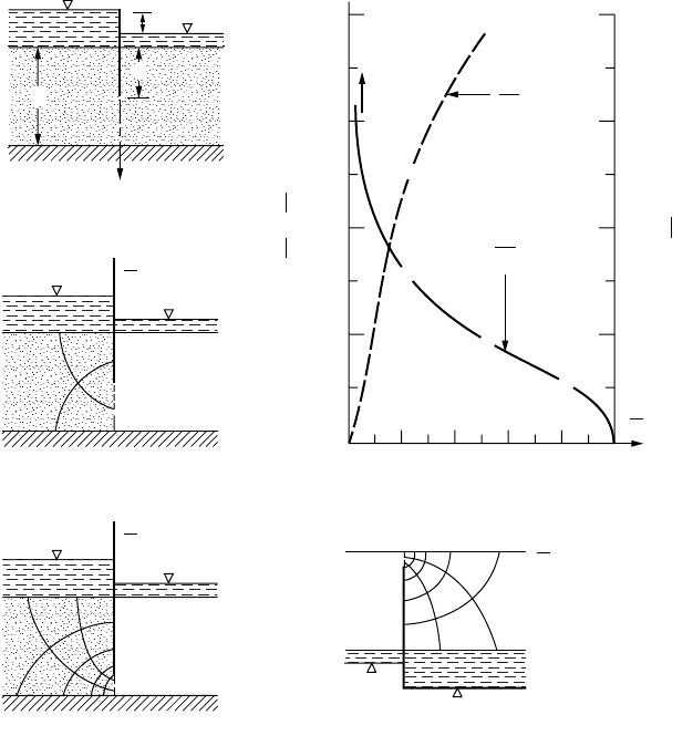
Example 18.3

Using ﬂow nets obtain a plot of Q/kh as a function of the ratio s/T for the single impervious sheetpile

shown in Fig. 18.10(a).

FIGURE 18.9 Example of ﬂow regime.

= 0

Coarse

screen

y =

y = 0

Coarse

screen

18-12 The Civil Engineering Handbook, Second Edition

Solution. We ﬁrst note that the section is symmetrical about the y axis, hence only one-half of a ﬂow

net is required. Values of the ratio s/T range from 0 to 1, with 0 indicating no penetration and 1 complete

cutoff. For s/T = 1, Q/kh = 0 [see point a in Fig. 18.10(b)]. As the ratio of s/T decreases, more ﬂow

channels must be added to maintain curvilinear squares and, in the limit as s/T approaches zero, Q/kh

becomes unbounded [see arrow in Fig. 18.10(b)]. If s/T = 1/2 [Fig. 18.10(c)], each streamline will

evidence a corresponding equipotential line in the half-strip; consequently, for the whole ﬂow region,

= 1/2 for s/T = 1/2 [point b in Fig. 18.10(b)]. Thus, without actually drawing a single ﬂow net, we

have learned quite a bit about the functional relationship between Q/kh and s/T. If Q/kh was known for

s/T = 0.8 we would have another point and could sketch, with some reliability, the portion of the plot

in Fig. 18.10(b) for s/T ≥ 0.5. In Fig. 18.10(d) is shown one-half of the ﬂow net for s/T = 0.8, which yields

the ratio of N

= 0.3 [point c in Fig. 18.10(b)]. As shown in Fig. 18.10(e), the ﬂow net for s/T = 0.8

can also serve, geometrically, for the case of s/T = 0.2, which yields approximately N

= 0.8 [plotted

as point d in Fig. 18.10(b)]. The portion of the curve for values of s/T close to 0 is still in doubt. Noting

that for s/T = 0, kh/Q = 0, we introduce an ordinate scale of kh/Q to the right of Fig. 18.10(b) and locate

on this scale the corresponding values for s/T = 0, 0.2, and 0.5 (shown primed). Connecting these points

(shown dotted) and obtaining the inverse, Q/kh, at desired points, the required curve can be had.

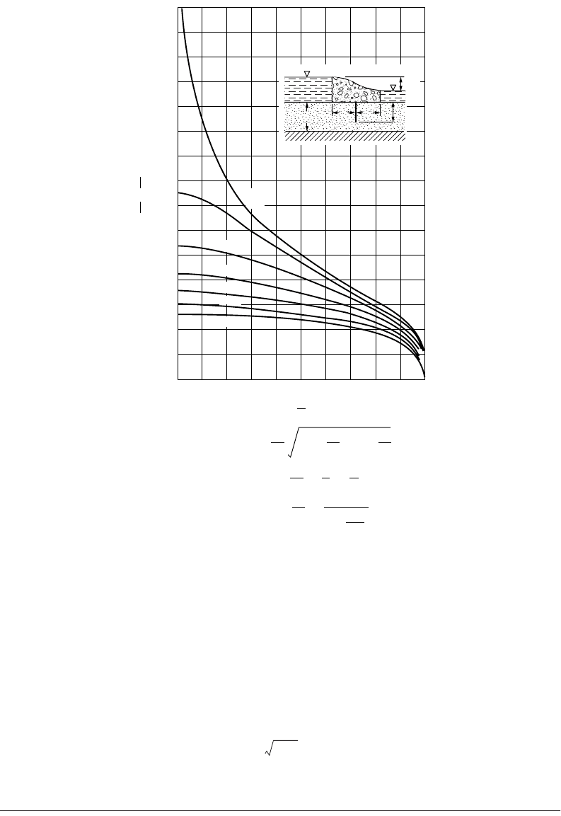
A plot giving the quantity of discharge (Q/kh) for symmetrically placed pilings as a function of depth

of embedment (s/T ), as well as for an impervious structure of width (2b/T ), is shown in Fig. 18.11. This

plot was obtained by Polubarinova-Kochina [1962] using a mathematical approach. The curve labeled

b/T = 0 applies for the conditions in Example 18.3. It is interesting to note that this whole family of

FIGURE 18.10 Example 18.3.

0 0.2 0.4 0.6 0.8 1.0

2.0

1.5

1.0

0.5

2.0

1.5

1.0

0.5

+b′

to ∞

curve

= 0.2

= 0.8

= 0.5

(

)

(

)

(

)

(

)

(

)

+ d′

Groundwater and Seepage 18-13

curves can be obtained, with reasonable accuracy (at least commensurate with the determination of the

coefﬁcient of permeability, k), by sketching only two additional half ﬂow nets (for special values of b/T ).

It was tacitly assumed in the foregoing that the medium was homogeneous and isotropic (k

= k

Had isotropy not been realized, a transformation of scale (with x and y taken as the directions of maximum

and minimum permeability, respectively) in the y direction of Y = y(k

)

1/2

or in the x direction of X =

x(k

)

1/2

would render the system as an equivalent isotropic system [for details, see Harr, 1962, p. 29].

After the ﬂow net has been established, by applying the inverse of the scaling factor, the solution can be

had for the anisotropic system. The quantity of discharge for a homogeneous and anisotropic section is

(18.26)

18.4 Method of Fragments

In spite of its many uses, a graphical ﬂow net provides the solution for a particular problem only. Should

one wish to investigate the inﬂuence of a range of characteristic dimensions (such as is often the case in

FIGURE 18.11 Quantity of ﬂow for given geometry.

1.5

1.4

1.3

1.2

1.1

1.0

0.9

0.8

0.7

0.6

0.5

0.4

0.3

0.2

0.1

0 0.1 0.2 0.3 0.4 0.5 0.6 0.7 0.8 0.9 1.0

= 0

0.25

0.50

0.75

1.00

1.25

1.50

= cos

tanh

+ tan

for

≤ 0.3, = In

−π

for

≤ 0.9, =

2 In

( )

2Φ

------

18-14 The Civil Engineering Handbook, Second Edition

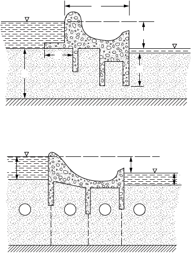
a design problem), many ﬂow nets would be required. Consider, for example, the section shown in

Fig. 18.12, and suppose we wish to investigate the inﬂuence of the dimensions A, B, and C on the

characteristics of ﬂow, all other dimensions being ﬁxed. Taking only three values for each of these

dimensions would require 27 individual ﬂow nets. As noted previously, a rough ﬂow net should always

be drawn as a check. In this respect it may be thought of as being analogous to a free-body diagram in

mechanics, wherein the physics of a solution can be examined with respect to satisfying conditions of

necessity.

An approximate analytical method of solution, directly applicable to design, was developed by Pav-

lovsky in 1935 [Pavlovsky, 1956] and was expanded and advanced by Harr [1962, 1977]. The underlying

assumption of this method, called the method of fragments, is that equipotential lines at various critical

parts of the ﬂow region can be approximated by straight vertical lines (as, for example, the dotted lines

in Fig. 18.13) that divide the region into sections or fragments. The groundwater ﬂow region in Fig. 18.13

is shown divided into four fragments.

Suppose, now, that one computes the discharge in the ith fragment of a structure with m such fragments

(18.27)

where h

is the head loss through the ith fragment and F

is the dimensional form factor in the ith fragment,

= N

in Eq. (18.25). Then, as the discharge through all fragments must be the same,

whence

FIGURE 18.12 Example of complicated structure.

FIGURE 18.13 Four fragments.

1234

-------=

--------

------- L

---------=====

----

Groundwater and Seepage 18-15

and

(18.28)

where h (without subscript) is the total head loss through the section. By similar reasoning, the head

loss in the ith fragment can be calculated from

(18.29)

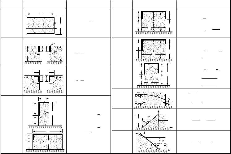
Thus, the primary task is to implement this method by establishing a catalog of form factors. Following

Pavlovsky, the various form factors will be divided into types. The results are summarized in tabular

form, Fig. 18.14, for easy reference. The derivation of the form factors is well documented in the literature

[Harr 1962, 1977].

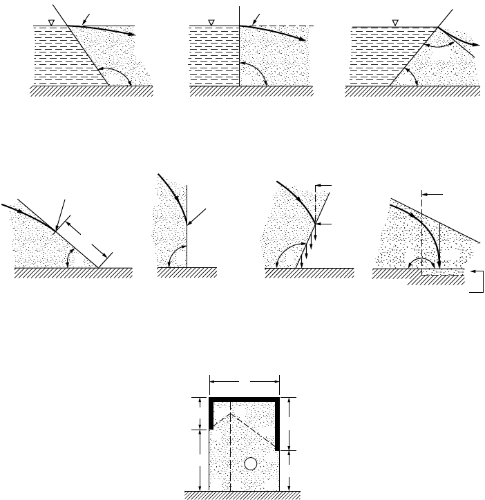
Various entrance and emergence conditions for type VIII and IX fragments are shown in Fig. 18.15.

Brieﬂy, for the entrance condition, when possible the free surface will intersect the slope at right angles.

However, as the elevation of the free surface represents the level of available energy along the uppermost

streamline, at no point along the curve can it rise above the level of its source of energy, the headwater

elevation. At the point of emergence the free surface will, if possible, exit tangent to the slope [Dachler,

1934]. As the equipotential lines are assumed to be vertical, there can be only a single value of the total

head along a vertical line, and, hence, the free surface cannot curve back on itself. Thus, where unable

to exit tangent to a slope, it will emerge vertical.

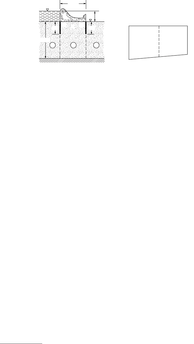
To determine the pressure distribution on the base of a structure (such as that along C ¢CC ¢¢) in

Fig. 18.16, Pavlovsky assumed that the head loss within the fragment is linearly distributed along the

impervious boundary. Thus, in Fig. 18.16, if h

is the head loss within the fragment, the rate of loss along

E¢C ¢CC ¢¢E ¢¢ will be

FIGURE 18.14 Summary of fragment types and form factors.

Fragment

type

Fragment

type

III

VIII

VII

Illustration Illustration

s''

b''

a''

45°

Streamline

45°

(1 + In )

cotβ

(1 + )

−

cot α

−

Φ =

Φ = In

Φ =

(1 +

)

−

Φ = In

Form factor, Φ (

is head

loss through fragment)

Form factor, Φ (

is head

loss through fragment)

≤ 2

Φ = 2 In (1 + )

− 2

≥ 2

Φ = 2 In (1 + ) +

≤

≥

′ +

′′:

Φ = In [(1 + ) +

′

−

(

′ +

′′)

(1 + )]

′′

( ), Fig. 17.11

Φ =

( ), Fig. 17.11

≤

′ +

′′:

Φ = In [(1 + )

′

(

′ −

′′)

(1 + )]

′′

−

(

′ −

′′)

where

i 1=

-------------------

----------=

18-16 The Civil Engineering Handbook, Second Edition

(18.30)

Once the total head is known at any point, the pressure can easily be determined by subtracting the

elevation head, relative to the established (tailwater) datum.

Example 18.4

For the section shown in Fig. 18.17(a), estimate (a) the discharge and (b) the uplift pressure on the base

of the structure.

Solution. The division of fragments is shown in Fig. 18.17. Regions 1 and 3 are both type II fragments,

and the middle section is of type V with L = 2s. For regions 1 and 3, we have, from Fig. 17,11, with b/T =

0, F

= F

= 0.78.

For region 2, as L = 2s, F

= 2 ln (1+18/36) = 0.81. Thus, the sum of the form factors is

and the quantity of ﬂow (Eq. 18.28) is Q/k = 18/2.37 = 7.6 ft.

FIGURE 18.15 Entrance and emergence conditions.

FIGURE 18.16 Illustration of Eq. (18.30).

Horizontal Horizontal

Tangent

Vertical

Drain

Tangent

vertical

Surface

of seepage

β < 90°β = 90°β > 90°

α > 90°α = 90°α < 90°

β = 180°

αα α′

90°

(

)

(

)

′

′′

′

C′ C

′′

C′′

O′

E′

45°

O′′

E′′

45°

Ls¢ s≤++

------------------------=

0.78 0.81 0.78++ 2.37==

Groundwater and Seepage 18-17

For the head loss in each of the sections, from Eq. (18.29) we ﬁnd

Hence the head loss rate in region 2 is (Eq. 18.30)

and the pressure distribution along C ¢CC ¢¢ is shown in Fig. 18.17(b).

Example 18.5

Estimate the quantity of discharge per foot of structure and the point where the free surface begins under

the structure (point A) for the section shown in Fig. 18.18(a).

Solution. The line AC in Fig. 18.18(a) is taken as the vertical equipotential line that separates the ﬂow

domain into two fragments. Region 1 is a fragment of type III, with the distance B as an unknown quantity.

Region 2 is a fragment of type VII, with L = 25 – B, h

= 10 ft, and h

= 0. Thus, we are led to a trial-and-

error procedure to ﬁnd B. In Fig. 18.18(b) are shown plots of Q/k versus B/T for both regions. The common

point is seen to be B = 14 ft, which yields a quantity of ﬂow of approximately Q = 100k/22 = 4.5k.

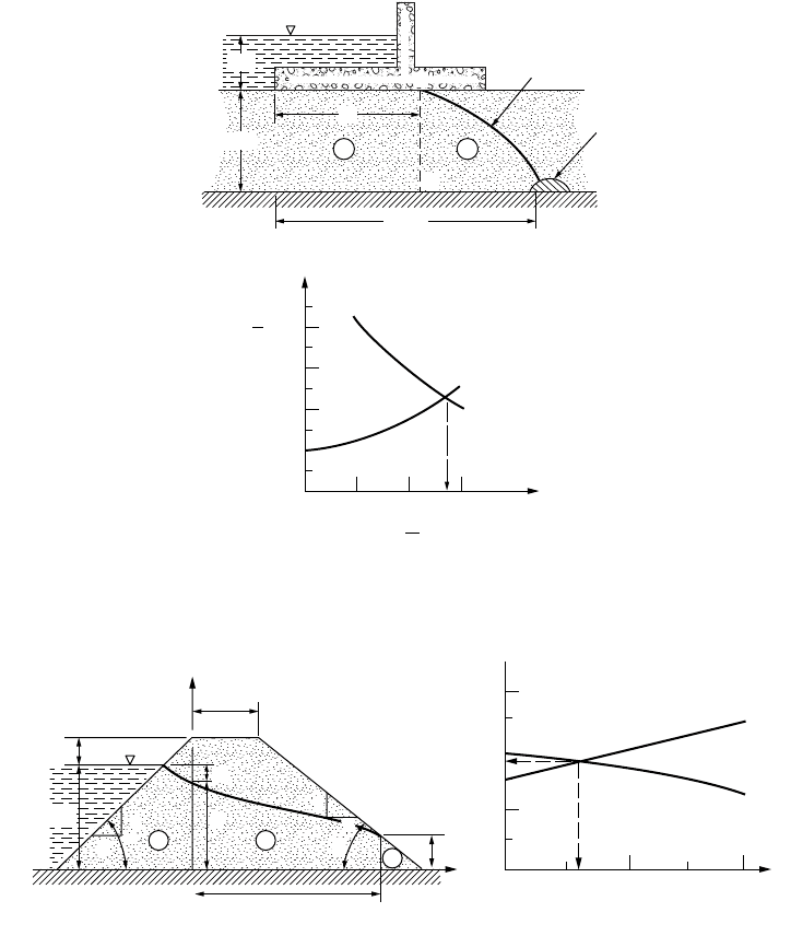
Example 18.6

Determine the quantity of ﬂow for 100 ft of the earth dam section shown in Fig. 18.19(a), where k =

0.002 ft/min.

Solution. For this case, there are three regions. For region 1, a type VIII fragment h

= 70 ft, cot a = 3,

= 80 ft, produces

(18.31)

For region 2, a type VII fragment produces

(18.32)

FIGURE 18.17 Example 18.4.

For comparisons between analytical and experimental results for mixed fragments (conﬁned and unconﬁned

ﬂow) see Harr and Lewis [1965].

18 ft

27 ft

9 ft

C′ C′′

12 3

C′ CC′′

10.6g

9.0g

7.5g

(

)

(

)

0.78

2.37

----------

18() 5.9 ft== =

6.1ft=

6.1

------- 17%==

----

70 h–

--------------

80 h–

--------------

ln=

----

–

---------------=

18-18 The Civil Engineering Handbook, Second Edition

With tailwater absent, h

= 0, the ﬂow in region 3, a type IX fragment, with cot b = 3 produces

(18.33)

Finally, from the geometry of the section, we have

(18.34)

The four independent equations contain only the four unknowns, h, a

, Q/k, and L, and hence provide

a complete, if not explicit, solution.

FIGURE 18.18 Example 18.5.

FIGURE 18.19 Example 18.6.

Free surface

Drain

25 ft

0 0.5 1.0 1.5

(

)

(

)

=14 ft

8 ft

10 ft

(

)

(

)

20 ft

10 ft

= 70 ft

(

)(

)

= 18.3 ft

= 52.7 ft

Eq. (17.38)

Eq. (17.36)

55 60

----

----=

L 20

cot h

–[]+ 20 3 80 a

–[]+==

Groundwater and Seepage 18-19

Combining Eqs. (18.32) and (18.33) and substituting for L in Eq. (18.34), we obtain, in general (b =

crest width),

(18.35)

and, in particular,

(18.36)

Likewise, from Eqs. (18.31) and (18.33), in general,

(18.37)

and, in particular,

(18.38)

Now, Eqs. (18.36) and (18.38), and (18.35) and (18.37) in general, contain only two unknowns (a

and h),

and hence can be solved without difﬁculty. For selected values of h, resulting values of a

are plotted for

Eqs. (18.36) and (18.38) in Fig. 18.19(b). Thus, a

= 18.3 ft, h = 52.7 ft, and L = 205.1 ft. From Eq. (18.33),

the quantity of ﬂow per 100 ft is

18.5 Flow in Layered Systems

Closed-form solutions for the ﬂow characteristics of even simple structures founded in layered media

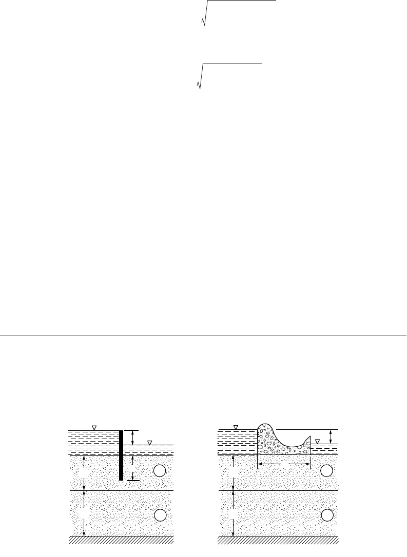
offer considerable mathematical difﬁculty. Polubarinova-Kochina [1962] obtained closed-form solutions

for the two layered sections shown in Fig. 18.20 (with d

= d

). In her solution she found a cluster of

parameters that suggested to Harr [1962] an approximate procedure whereby the ﬂow characteristics of

structures founded in layered systems can be obtained simply and with a great degree of reliability.

FIGURE 18.20 Examples of two-layered systems.

cot

------------ h

cot

------------ h

Ë¯

Êˆ

––+=

----- 80

----- 80+

Ë¯

Êˆ

–+=

cot

------------------ h

h–()

h–

--------------

ln=

70 h–()

80 h–

--------------

ln=

Q 100 2 10

3–

18.3

----------

¥¥¥ 1.22 ft

min§ 9.1 gal min§===

(

)(

)